Julia is a relatively new, free, and open-source programming language. It has a syntax similar to that of other popular programming languages such as MATLAB and Python, but it boasts being able to achieve C-like speeds.

Unlike other languages that focus on technical computing, Julia does not require users to vectorize their code (i.e., to have one version of a function that operates on scalar values and another version that operates on arrays). Instead, Julia provides a built-in mechanism for vectorizing functions: broadcasting.

Broadcasting is useful in Julia for several reasons, including:

• It allows functions that operate on scalar values (e.g., cos(π)) to operate elementwise on an array of values, eliminating the need for specialized, vectorized versions of those functions.
• It allows for more efficient memory allocation in certain situations. For example, suppose we have a function, func, and we want to compute func(1, 2) and func(1, 3). Instead of broadcasting on [1, 1] and [2, 3], we can broadcast on 1 and [2, 3], avoiding the memory allocation for [1, 1].

On top of that, Julia provides a very convenient syntax for broadcasting, making it so anyone can easily use broadcasting in their code.

In this post, we will learn what broadcasting is, and we will see several examples of how to effectively use broadcasting.

This post assumes you already have Julia installed. If you haven't yet, check out our earlier post on how to install Julia.

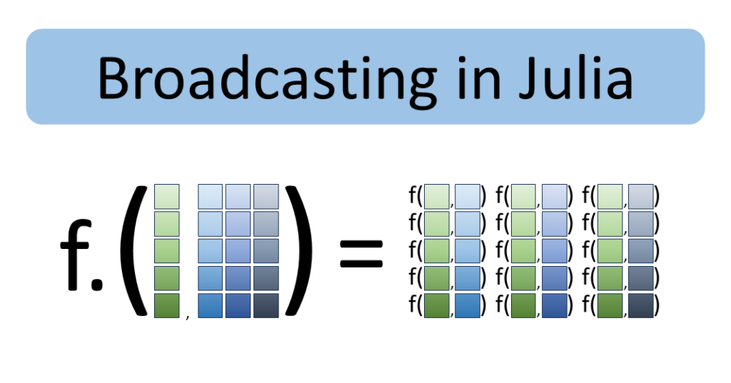
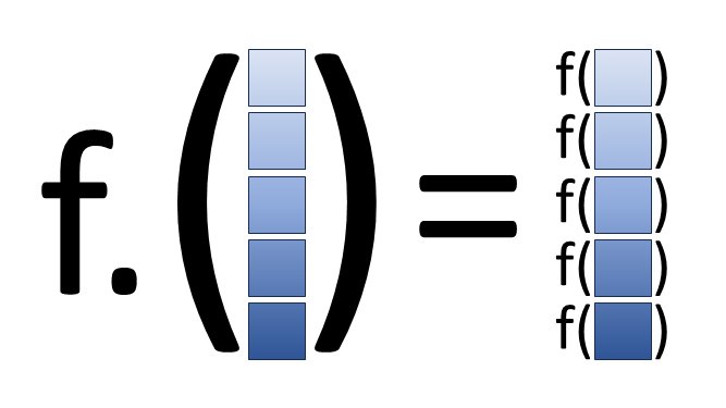
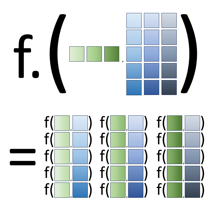
What Is Broadcasting?

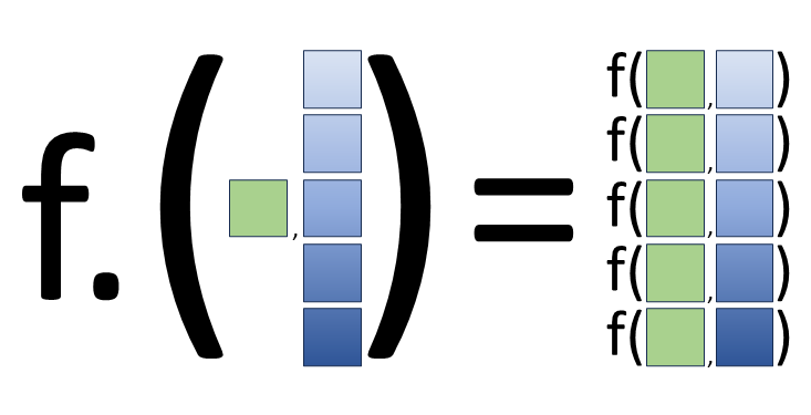
Broadcasting essentially is a method for calling functions elementwise while virtually copying inputs so that all inputs have the same size. (For example, if two inputs to a broadcasted function f are 1 and [1, 2, 3], the first input is treated as if it is [1, 1, 1] but without actually allocating memory for an array. Then the function is applied to each pair of inputs: f(1, 1), f(1, 2), and f(1, 3).)

If that definition doesn't make sense right now, don't worry, the examples below will help illustrate.

The Dot Syntax

The first thing to know about broadcasting is that it is very convenient to use.

All you need to do is add dots.

For example, if you want to take the square root of a collection of values, just add a dot (.):

julia> sqrt.([1, 4, 9]) # Notice the dot after `sqrt`
3-element Vector{Float64}:
 1.0
 2.0
 3.0

Vectorizing Operators and Functions

As stated earlier, Julia doesn't require vectorized versions of functions. In fact, many functions don't even have methods that take array inputs. Take sqrt for example:

julia> sqrt([1, 4, 9]) # No dot after `sqrt`
ERROR: MethodError: no method matching sqrt(::Vector{Int64})

So, even though sqrt doesn't have a vectorized version explicitly defined, the dot syntax still allows sqrt to be applied elementwise. The same applies to other functions and operators:

julia> [1, 2, 3] ^ 3 # No dot
ERROR: MethodError: no method matching ^(::Vector{Int64}, ::Int64)

julia> [1, 2, 3] .^ 3 # With dot
3-element Vector{Int64}:
  1
  8
 27

julia> uppercase(["hello", "world"]) # No dot
ERROR: MethodError: no method matching uppercase(::Vector{String})

julia> uppercase.(["hello", "world"]) # With dot
2-element Vector{String}:
 "HELLO"
 "WORLD"

Vectorization even works with user-defined functions:

julia> myfunc(x) = x * 2
myfunc (generic function with 1 method)

julia> myfunc.([1, 2])
2-element Vector{Int64}:
 2
 4

Note that some functions do have methods that operate on arrays, so be careful when deciding whether a function should apply elementwise. Take cos as an example:

julia> A = [0 π; π/2 π/6];

julia> cos(A) # Matrix cosine, *not* elementwise cosine
2x2 Matrix{Float64}:
 -0.572989  -0.285823
 -0.142912  -0.620626

julia> cos.(A) # Add a dot for computing the cosine elementwise
2x2 Matrix{Float64}:
 1.0          -1.0
 6.12323e-17   0.866025

Broadcasting with Multiple Inputs

Broadcasting gets more interesting when multiple inputs are involved. Let's use addition (+) as an example.

We can add a scalar to each element of an array:

julia> [1, 2, 3] .+ 10
3-element Vector{Int64}:
 11
 12
 13

julia> 10 .+ [1, 2, 3]
3-element Vector{Int64}:
 11
 12
 13

We can also sum two arrays elementwise:

julia> [1, 2, 3] .+ [10, 20, 30]
3-element Vector{Int64}:
 11
 22
 33

Broadcasting even works with arrays of different sizes. The only requirement is that non-singleton dimensions must match across inputs.

julia> [1 2 3; 4 5 6] .+ [10, 20] # Sizes: (2, 3) and (2,)
2x3 Matrix{Int64}:
 11  12  13
 24  25  26

julia> [1 2 3; 4 5 6] .+ [10 20] # Sizes: (2, 3) and (1, 2)
ERROR: DimensionMismatch: arrays could not be broadcast to a common size; got a dimension with lengths 3 and 2

julia> [1 2 3; 4 5 6] .+ [10 20 30] # Sizes: (2, 3) and (1, 3)
2x3 Matrix{Int64}:
 11  22  33
 14  25  36

In the first example ([1 2 3; 4 5 6] .+ [10, 20]), the column vector [10, 20] was added to each column of the matrix, while in the second working example ([1 2 3; 4 5 6] .+ [10 20 30]), the row vector [10 20 30] was added to each row of the matrix.

Treating Inputs as Scalars

Sometimes, it is useful to broadcast over only a subset of the inputs. For example, suppose we have a function that scales an input matrix:

julia> myfunc2(X, a) = X * a
myfunc2 (generic function with 1 method)

Suppose we want to scale a given matrix by several different scale factors. The result should be an array of matrices, one matrix for each scale factor applied. We might try to use broadcasting:

julia> X = [1 2; 3 4]; a = [10, 20];

julia> myfunc2.(X, a)
2x2 Matrix{Int64}:
 10  20
 60  80

But the result is just one matrix! We have one matrix because we broadcasted over a and X, not just a. In this case, we need to wrap X in a single-element Tuple:

julia> myfunc2.((X,), a)
2-element Vector{Matrix{Int64}}:
 [10 20; 30 40]
 [20 40; 60 80]

Now we have the result we want: an array where the first entry is X scaled by a[1] and the second entry is X scaled by a[2].

So, whenever you need to treat an input as a scalar for broadcasting purposes, just wrap it in a Tuple.

Broadcasting with Dictionaries and Strings

Dictionaries and strings may act differently than expected in broadcasting, so let's clarify some things here.

First, attempting to broadcast over a dictionary will throw an error:

julia> d = Dict("key1" => "hello", "key2" => "world")
Dict{String, String} with 2 entries:
  "key2" => "world"
  "key1" => "hello"

julia> println.(d)
ERROR: ArgumentError: broadcasting over dictionaries and `NamedTuple`s is reserved

There are different solutions depending on the context. For example:

• Treat the dictionary as a scalar:

  julia> println.((d,)); # Note that `d` is wrapped in a `Tuple`
  Dict("key2" => "world", "key1" => "hello")
  

• Broadcast over the values explicitly:

  julia> println.(values(d));
  world
  hello
  

Regarding strings, strings are treated as scalars, not as collections of characters. For example:

julia> string.("string", [1, 2])
2-element Vector{String}:
 "string1"
 "string2"

(The above would have errored if strings were not treated as scalars, because length("string") is 6, whereas length([1, 2]) is 2.)

To broadcast over the characters in a string, use collect:

julia> string.(collect("string"), 1:6)
6-element Vector{String}:
 "s1"
 "t2"
 "r3"
 "i4"
 "n5"
 "g6"

Summary

In this post, we learned what broadcasting is, and we saw several examples of how to effectively use broadcasting to apply functions elementwise.

Have any further questions about broadcasting? Feel free to ask them in the comments below!

Does broadcasting make sense now? Move on to the next post to learn about Julia's type system! Or, feel free to take a look at our other Julia tutorial posts!

Additional Links

• Julia documentation about broadcasting:
  • Vectorized operators
  • Vectorized functions
  • Broadcasting on arrays
• Installing Julia and VS Code - A Comprehensive Guide
  • How-to guide for installing Julia and VS Code.
• Understanding the Julia Type System
  • Introduction to how Julia handles types.