Julia is a relatively new, free, and open-source programming language. It has a syntax similar to that of other popular programming languages such as MATLAB and Python, but it boasts being able to achieve C-like speeds.

Julia provides several useful data structures for storing and manipulating data. Some of these data structures, like arrays and dictionaries, are ubiquitous in Julia code because of their usefulness and wide applicability. Others, like sets, have more limited uses but nevertheless still are useful data structures.

In this post, we will learn about arrays, dictionaries, and sets in Julia. We will discuss how to construct them and describe various functions for working with and manipulating them.

This post assumes you already have Julia installed. If you haven't yet, check out our earlier post on how to install Julia.

Arrays

One of the most basic and ubiquitous data structures is the array. Arrays are used for storing values, iterating through values, and even representing mathematical vectors and matrices.

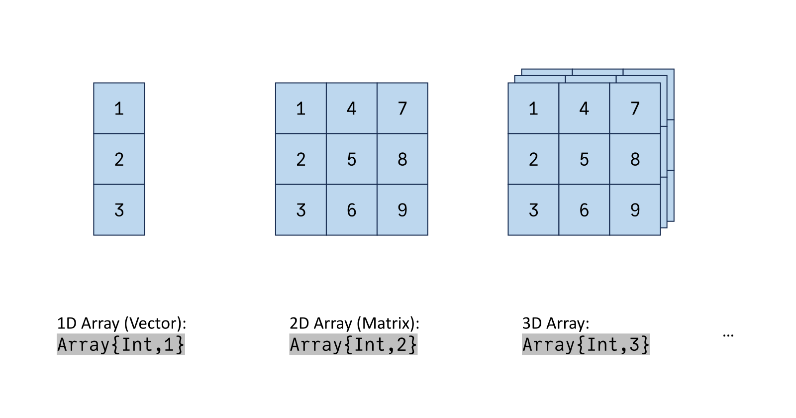
The basic array type in Julia is Array{T,N}, where T is the type of the elements in the array (or an abstract supertype of the elements if not all elements are of the same type), and N is the number of array dimensions. For example, a list of strings would be of type Array{String,1}, while a matrix of numbers would be of type Array{Float64,2}.

Constructing Arrays

There are various ways to construct arrays. One common way is to construct an array directly from the values it will contain:

julia> ["some", "strings"]
2-element Vector{String}:
 "some"
 "strings"

julia> [1 2; 3 4]
2x2 Matrix{Int64}:
 1  2
 3  4

(Note that Vector{T} is equivalent to Array{T,1} and that Matrix{T} is equivalent to Array{T,2}.)

Example arrays

Another common way to construct arrays is using array comprehensions. An array comprehension creates an array by looping through a collection of values and computing an array element for each value. For example, the following creates an array containing the squares of the first five natural numbers:

julia> [x^2 for x = 1:5]
5-element Vector{Int64}:
  1
  4
  9
 16
 25

Multidimensional comprehensions also exist:

julia> [(x - 2)^2 + (y - 3)^2 <= 1 for x = 1:3, y = 1:5]
3x5 Matrix{Bool}:
 0  0  1  0  0
 0  1  1  1  0
 0  0  1  0  0

We can also create uninitialized arrays, either by passing undef to the array constructor or by calling similar:

julia> Array{Int,1}(undef, 1)
1-element Vector{Int64}:
 6303840

julia> similar([1.0, 2.0])
2-element Vector{Float64}:
 6.94291544947797e-310
 6.94291610129443e-310

(Note that the seemingly random numbers above come from whatever bits happen to be set in the memory allocated for the arrays.)

To create an array of zeros, call zeros:

julia> zeros(2, 3)
2x3 Matrix{Float64}:
 0.0  0.0  0.0
 0.0  0.0  0.0

Inspecting Arrays

Information about an array can be obtained using various functions.

length gives the number of elements in an array:

julia> length([1, 2, 3])
3

julia> length(zeros(2, 3))
6

size(x) gives the size of x, while size(x, d) gives the size of the dth dimension:

julia> size([1, 2, 3])
(3,)

julia> size(zeros(2, 3))
(2, 3)

julia> size(zeros(2, 3), 2)
3

ndims gives the number of dimensions of an array:

julia> ndims(zeros(1, 2, 3, 4, 5, 6))
6

And eltype gives the type of the elements of an array:

julia> eltype(["two", "strings"])
String

julia> eltype([2, "different types"])
Any

Array Operations

Accessing array elements is achieved using brackets:

julia> a = [10, 20, 30];

julia> a[2]
20

(Note that arrays use one-based indexing in Julia.)

A similar syntax is used to modify the contents of an array:

julia> a[1] = 0
0

julia> a
3-element Vector{Int64}:
  0
 20
 30

Use commas (,) to separate indexes for different dimensions, and use a colon (:) to select all the values along a dimension:

julia> m = [1 2; 3 4]
2x2 Matrix{Int64}:
 1  2
 3  4

julia> m[1,2]
2

julia> m[:,1]
2-element Vector{Int64}:
 1
 3

Multiple indexes can be provided:

julia> a[[1, 3]]
2-element Vector{Int64}:
  0
 30

To assign a single value to multiple array locations, use broadcasting:

julia> a[2:3] .= 0
2-element view(::Vector{Int64}, 2:3) with eltype Int64:
 0
 0

julia> a
3-element Vector{Int64}:
 0
 0
 0

Arrays are also iterable, meaning we can loop through the values of an array:

julia> words = ["this", "is", "a", "sentence"];

julia> for w in words
           println(w)
       end
this
is
a
sentence

Arrays as Stacks/Queues/Dequeues

Julia also provides some functions that allow arrays to be used in a similar way as stacks, queues, and dequeues. For example, push!(array, x) inserts x at the end of an array, and pop!(array) removes the last element of an array. Similarly, pushfirst! and popfirst act on the beginning of an array.

Ranges

Ranges are another useful type of array, often used for looping and array indexing.

The simplest syntax for creating a range is a:b, which creates a range that starts at a and includes all values a + 1, a + 2, etc., as long as a + n <= b. For example, 1:5 contains 1, 2, 3, 4, and 5, while 1.0:2.5 contains 1.0 and 2.0.

A step size, s, can also be specified, as in a:s:b. In this case, the spacing between values in the range is s instead of 1.

To create a range of N points between a and b, inclusive, use range(a, b, N).

Unlike Arrays, ranges are immutable, meaning their elements can't be modified. If modifying an element of a range is necessary, it must first be converted into an Array by calling collect:

julia> r = 1:2
1:2

julia> r[1] = 10
ERROR: CanonicalIndexError: setindex! not defined for UnitRange{Int64}

julia> r_arr = collect(r)
2-element Vector{Int64}:
 1
 2

julia> r_arr[1] = 10; r_arr
2-element Vector{Int64}:
 10
  2

That concludes our discussion of arrays, so now let's move on to dictionaries.

Dictionaries

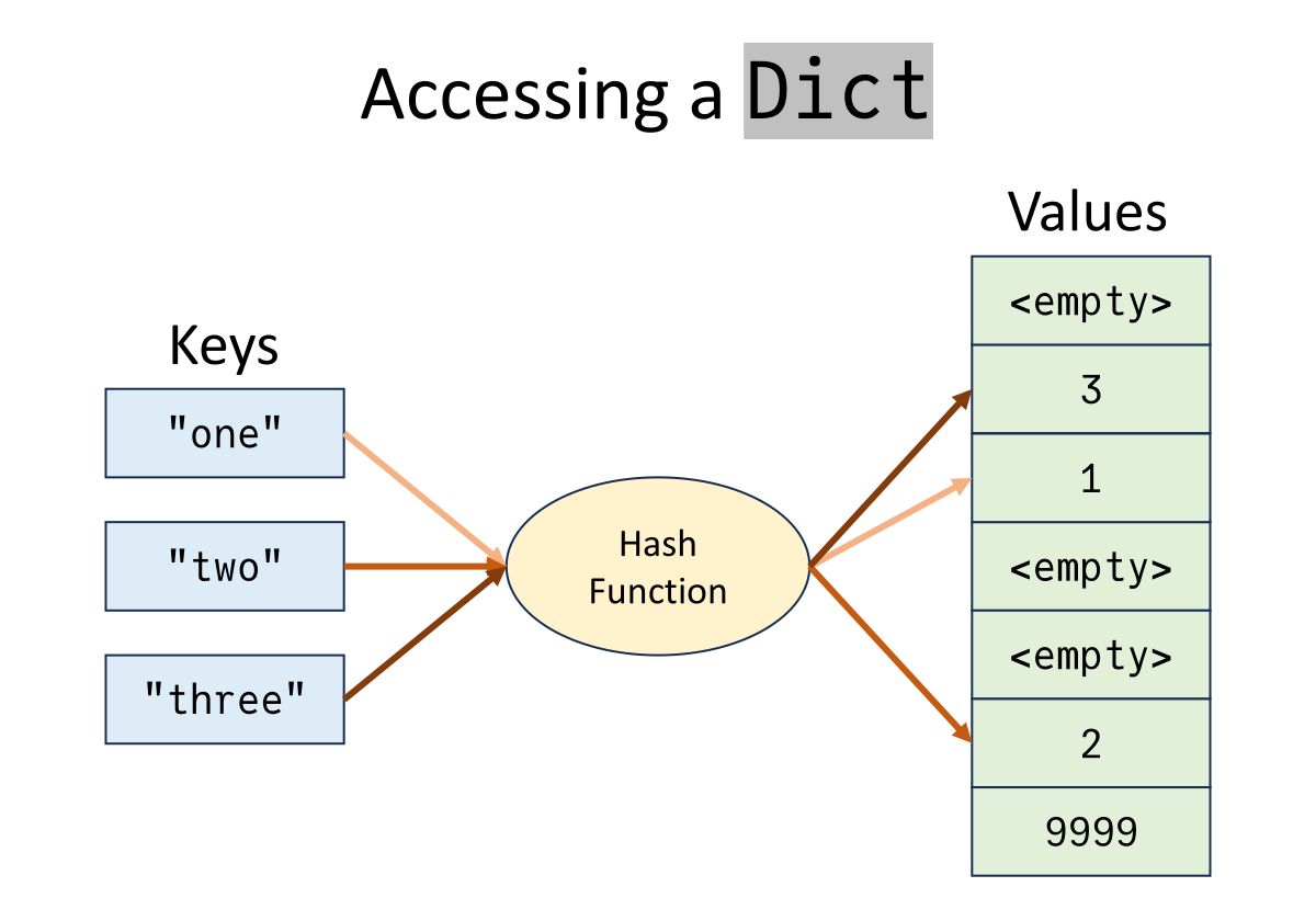
Another very common data structure is the dictionary. A dictionary is a mapping from keys to values: give a dictionary a key, and it will return the value associated with that key (if present).

In Julia, dictionaries are of type Dict{K,V}, where K is the type of the keys, and V is the type of the values.

Dictionaries are constructed by providing key-value pairs:

julia> d = Dict("key1" => 1, "key2" => 2, "key3" => 3)
Dict{String, Int64} with 3 entries:
  "key2" => 2
  "key3" => 3
  "key1" => 1

(Note that a => b creates a Pair in Julia.)

Indexing a dictionary uses the same syntax as indexing an array, just using keys instead of array indexes:

julia> d["key2"]
2

Accessing a dictionary

Use haskey to check for the presence of a key:

julia> haskey(d, "key3")
true

julia> haskey(d, "nope")
false

Dictionaries can also be updated:

julia> d["key1"] = 9999
9999

julia> d["newkey"] = -9999
-9999

julia> d
Dict{String, Int64} with 4 entries:
  "key2"   => 2
  "key3"   => 3
  "key1"   => 9999
  "newkey" => -9999

Use delete!(dict, key) to delete the mapping for the given key, if present.

We can also iterate through the keys and/or values of a dictionary:

Iterating keys: for k in keys(dict)
Iterating values: for v in values(dict)
Iterating both: for (k, v) in dict

That wraps up our discussion of dictionaries, so now we will move on to sets.

Sets

A set is a collection of unique elements. In Julia, sets are of type Set{T}, where T is the type of the elements of the set. Sets are useful for their efficient set operations, such as membership testing, union, and intersect.

Create an empty set of Float64 values as follows:

julia> s = Set{Float64}()
Set{Float64}()

Use push! to add values to the set, noticing that the set changes only if the value does not already exist in the set:

julia> push!(s, 1.0);

julia> push!(s, 1.2);

julia> push!(s, 3.14)
Set{Float64} with 3 elements:
  1.2
  3.14
  1.0

julia> push!(s, 1.0)
Set{Float64} with 3 elements:
  1.2
  3.14
  1.0

Use union to take the union of two sets:

julia> t = Set([1.0, 2.0])
Set{Float64} with 2 elements:
  2.0
  1.0

julia> r = s ∪ t # type \cup<tab> to get the union symbol
Set{Float64} with 4 elements:
  1.2
  2.0
  3.14
  1.0

(Note that s ∪ t == union(s, t).)

Use intersect to take the intersection of two sets:

julia> r ∩ t # type \cap<tab> to get the intersection symbol
Set{Float64} with 2 elements:
  2.0
  1.0

(Note that s ∩ t == intersect(s, t).)

Finally, we can check if an element belongs to a set with in:

julia> 1.0 ∈ r # type \in<tab> to get the "is an element of" symbol
true

(Note that ∈ and in are interchangeable here.)

And with that, we conclude our overview of some important Julia data structures.

Summary

In this post, we learned about a few data structures that Julia provides: arrays, dictionaries, and sets. We learned how to construct them and how to work with and manipulate them.

What are the most useful data structures you have used? Let us know in the comments below!

Have a better understanding of Julia's basic data structures? Move on to the next post to learn about multiple dispatch, one of Julia's most distinctive features! Or, feel free to take a look at our other Julia tutorial posts!

Additional Links

Julia Documentation: Arrays
- Additional information about arrays.
Julia Documentation: Collections and Data Structures
- Additional information about arrays, dictionaries, and sets.
DataStructures.jl
- Package providing several more data structures, including priority queues, binary heaps, trees, and more. See the README for a complete list.

Basic Data Structures Explained

Understand core Julia data structures - arrays, dictionaries, and sets.

Table of contents