This post is a cleaned-up transcript of the JuliaCon 2025 talk Integrating Julia and MATLAB: Julia and MATLAB Can Coexist by Steven Whitaker. Check out the submission page for the talk abstract and summary. To download a PowerPoint of the talk slides, click here.

Introduction

Thank you for the introduction. I'm going to be talking about Julia-MATLAB integration. I'll start by talking about why we might want to do this. Why not just stick with MATLAB^® or why not transition entirely to Julia? I'll talk about how to actually do the integration and I'll walk through an example model. I'll show you the MATLAB code, show how it needs to be translated to Julia and then reintegrated back into the MATLAB workflow that we're working with. And I'll demonstrate some benchmark results from before and after doing the Julia-MATLAB integration.

MATLAB Is Everywhere, Julia Is Fast

To begin, I do want to say that from our perspective MATLAB is great software. It's used by businesses and people all over the world, and it has withstood the test of time. MATLAB has excellent tooling and documentation. It has been the go-to for scientific computing and engineering, and it is ubiquitous in modeling and simulation. By a quick raise of hands, who here has written a model or a function in MATLAB? I think literally everyone (in the JuliaCon audience). Me too. Engineers have had time to amass decades worth of MATLAB models and workflows, which is to say MATLAB isn't going anywhere.

But is MATLAB the best option in all cases? Now, there's this trade-off between speed and what I'll call reputation. MATLAB has an incredibly good reputation. It has excellent tooling. It's robust and it has a ton of other awesome features. It has gained a reputation for being reliable and it is an established industry standard. Large companies may have hundreds of MATLAB models and thousands upon thousands of lines of MATLAB code. But that makes it impractical to switch all this MATLAB code entirely over to Julia all at once.

However, there may be instances where MATLAB isn't the best choice to use. For example, if you have performance critical or large-scale models where speed is absolutely paramount, a language like Julia may be more suitable for those cases. Let's look at some concrete numbers.

Benchmark Comparisons

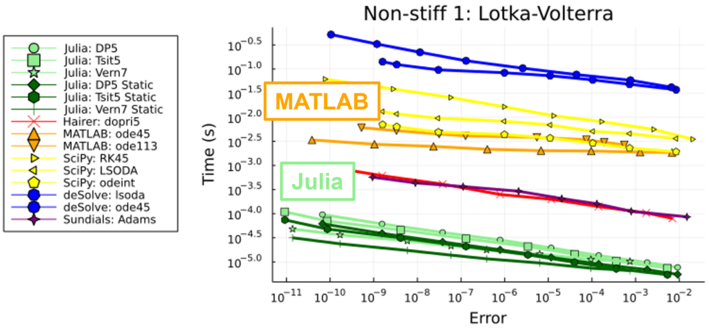
I pulled some benchmarks from the SciML benchmarks website. And as an aside for those of you who haven't heard about the SciML ecosystem, the Julia scientific machine learning ecosystem is incredible. So check it out if you haven't yet.

So what these benchmarks do is compare ODE solvers from various languages for various ODEs and just see how fast these ODE solvers compare. So for one example we have a non-stiff problem here. We're plotting how long it takes these ODE solvers to solve this non-stiff problem. The Julia solvers are in green, MATLAB in orange. And looking at this plot, we see that for this particular non-stiff problem, Julia is 10 to 1000 times faster than MATLAB.

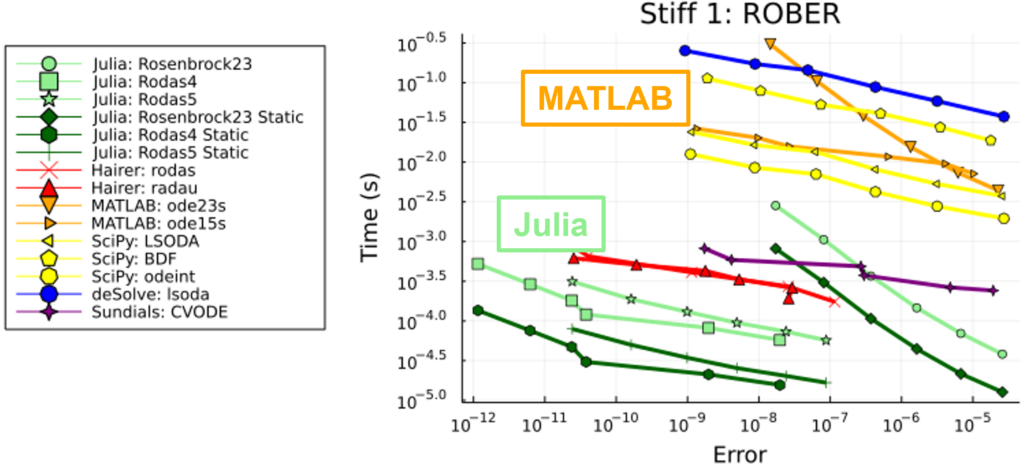
Now what about a stiff problem? Similar story for this particular stiff problem. Julia is 10 to 1000 times faster than MATLAB.

Now consider if your long simulations or parameter optimizations take hours or even days to run in MATLAB. You have to start asking yourself: is it worth using MATLAB when time is money? Does the reputation of MATLAB really outweigh the cost in time?

Introducing Julia with Minimal Disruptions

The key question is: How do we get Julia's speed but without rewriting all of our MATLAB code in Julia? How can we get that speed without major disruption, without completely retooling everything?

So another question: does anyone here by the raise of hands work with large MATLAB codebases? All right, a few of you (in the JuliaCon audience). Like I said, companies have had decades to mass tons of MATLAB code. And so if you're working at a company that has a large MATLAB codebase, if you use MATLAB every day, your colleagues use MATLAB every day, and, frankly, the code works, it runs, it gives the results that you need—these are all valid reasons for sticking with MATLAB. But the speed—Julia is fast! And some might say that Julia is the superior language. That's why we're here at JuliaCon—we want to use Julia!

The good news is that there is a way to introduce Julia into your MATLAB workflows, and you can do this with minimal disruption. You want to start small. Pinpoint the particular pain point in your MATLAB workflow and start targeting that area. You want to keep your existing MATLAB workflows intact. That way you help keep people on board with your project. But most importantly, you also want to show meaningful performance wins because that ultimately gets people's attention.

Example Model

For the rest of my talk, I will walk through the process of doing Julia-MATLAB integration using an example model. The example model that I'll use includes 50 equations and state variables along with 37 model parameters.

We'll also have discrete events and continuous events. For the discrete events, we will update one of the parameters at four specific time points along the simulation. An example of this in practice might be injecting a dose of medicine or modifying the thrust provided by a rocket.

We'll also have a continuous event where we modify a state variable when it reaches a certain value. A classic example is when modeling the velocity of objects that collide with boundaries. For example, if you drop a ball, that ball is going to fall until it hits the ground. And when it hits the ground, it doesn't keep falling. There's an event that occurs that causes the ball to bounce. That's the sort of thing that's captured by these continuous events.

For our example, we'll look at two problems of interest. One is just simply solving the ODE one time. How long does it take to do that? But then in practice, we don't normally solve an ODE a single time and then call it quits. Normally, we're solving ODEs many, many times. So, we're also going to look at doing a parameter sweep where we'll solve this example model ODE with about 200,000 different sets of model parameters and then choose the one to use in production.

Model Plots

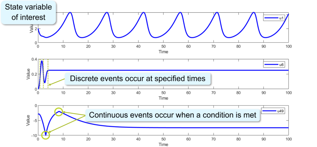
To illustrate this model a bit more, here are three of the state variables plotted over time. The first plot is a state variable of interest. This might represent the position of a mechanical part, or maybe it's the temperature of concrete or some other substance that we're modeling over time.

The second plot illustrates the discrete events. At these particular time points, we're changing one of the model parameters, and we see how that influences the time course for the state variable.

And then the third plot illustrates the continuous events where, when this state variable reaches a value of -10 or -2, we negate its derivative and we see how the time course is influenced as a result.

Looking back at the first state variable here, I'm plotting it for two different sets of model parameters. The first set of model parameters results in these large oscillations while the second set of model parameters has virtually no oscillations.

MATLAB ODE Solve Timing

The first question is how long did it take to solve this ODE one time so we could get this plot. Solving this ODE in MATLAB took about 20 milliseconds. Okay, so maybe that's not so bad.

Now, going back to this plot, like I mentioned, this state variable might represent the position of a mechanical part. And so if we have these oscillations, we can imagine that those oscillations cause wear on this mechanical part. And as a result, we would love to use the second set of model parameters so that there's less wear on that part, which means we don't have to replace it as often, which saves our company money. The problem is we don't know what those parameters are beforehand. Okay. So, what we'll do is pick 200,000 different sets of parameter values. We'll solve the ODE with each of those sets of parameter values and choose the parameter set that minimizes the oscillations so that we don't have to replace this part so often.

Now, if we do this parameter sweep in MATLAB, it takes about five hours to run on my laptop.

Now, if you run this exactly one time, maybe that's not such a huge deal. But if this is part of continuous integration or testing or if you do a parameter sweep for many different models and many different workflows, you can see how the time starts to add up quickly.

So, we want to see how Julia can fare in this situation. What we're going to do is we're going to take our MATLAB parameter sweep and translate that into Julia but then reconnect it into our MATLAB workflow.

Julia vs MATLAB for Simulations

The first thing to mention when converting from MATLAB to Julia is the syntax. MATLAB and Julia have a very similar syntax. MATLAB was the language that I used primarily before I started using Julia, and when I started learning Julia it almost didn't feel like I was learning a new language. That's how similar the syntax was to me.

In terms of the dynamics, Julia is designed for performance. In MATLAB, every time the ODE solver calls out to your dynamics function it has to allocate new memory to store the results of the computed state derivatives. Whereas in Julia, you can allocate that memory up front and then every time the ODE solver calls out to your dynamics function, it can reuse that memory, which boosts performance.

Events and Callbacks

I found that in Julia working with events and callbacks was more intuitive and easier to do. For this particular example, I could define them in fewer lines of code in Julia. Julia provides for better code organization and it also provides many pre-built callbacks that you can use out of the box.

So, looking more into events and callbacks: here's some example code in MATLAB and in Julia for defining events and callbacks.

%% MATLAB

% In events_func.m
v(n+1) = u(u49) + 2;
v(n+2) = u(u49) + 10;

% In callback_func.m
if any(ismember([n + 1, n + 2], ie))
    u(u50) = -u(u50);
end

# Julia

# In callbacks.jl
event1(u, t, integrator) = u[u49] + 2
event2(u, t, integrator) = u[u49] + 10
callback!(integrator) = integrator.u[u50] = -integrator.u[u50]
ContinuousCallback(event1, callback!)
ContinuousCallback(event2, callback!)

In MATLAB we have one file for the events and then a separate file for all the callbacks. Whereas in Julia we can define the events and the corresponding callbacks together in the same file which allows for better code organization.

Additionally, in MATLAB we have a single function that defines all of the events and then we have a single function that defines all of the callbacks. In Julia we can be more modular. We can define a single function per event, a single function per callback.

And then finally, in MATLAB there's more bookkeeping that we have to do on our own. We have to keep track of indexes of the events. We have to manually check if events occur and manually call the correct callbacks if those events occur. Whereas Julia takes care of all of that for us. In Julia, all we have to do is explicitly pair an event with its callback and then Julia takes care of the rest. Julia will check if the event occurs. It will then call the correct callback that you assigned it and we don't have to worry about that ourselves.

So again, I found that working with events and callbacks in Julia was more intuitive and easier to do.

Julia Is Easy to Learn

Now, another consideration when adopting a new software is how much learning you have to do to get up and running with it. I already mentioned the syntax. Julia syntax is similar to MATLAB, and so that isn't much of a barrier to entry.

Then there's also what packages are available and how quickly can I learn those packages. For this particular example I only needed to use two Julia packages to get it up and running. I used DiffEqCallbacks.jl for the events and callbacks and OrdinaryDiffEq.jl for setting up and solving the ODE.

And then perhaps more importantly: part of learning the package is going through its documentation and learning how to use the package from the documentation. So how good is the documentation?

Particularly for the SciML ecosystem, but also other ecosystems in Julia, the documentation is excellent. So if you look at the OrdinaryDiffEq.jl documentation it will clearly go through how to set up an ODE problem, how to solve it, and what options are available for solving. It also has a list of different solvers and shows you how to swap out different solvers with essentially just a single line of code change in Julia.

Then the DiffEqCallbacks.jl documentation is similarly good. It describes quite a few ready-to-use callbacks that you can use. There's the PresetTimeCallback for the discrete events at specific times. There are also more advanced callbacks such as those for step size control.

And then kind of the cherry on top for converting from MATLAB to Julia is there's one of the pages of the documentation that is a solver comparison. And so basically what it does is it lists the MATLAB solvers and then it says what are the corresponding Julia solvers you can use. So if in MATLAB you're using the ode45 solver, this web page will say, "okay, the corresponding Julia solver is DP5, but then there are also these other solvers you might want to try that might perform better."

So, the excellent documentation, the excellent package ecosystem and the similar syntax between Julia and MATLAB really makes transitioning from MATLAB to Julia a breeze.

Julia-MATLAB Integration Demo

Doing the actual integration we use the MATFrost.jl package. MATFrost.jl is a package that was developed by ASML. So, thank you to ASML for developing the package and open sourcing it for the Julia community to use. And I will illustrate the process of integrating Julia back into MATLAB via a live demo. So, I'm going to switch over to MATLAB.

% demo.m

[u0, tspan, p] = get_inputs();
[p_opt_indexes, grid_vals, lb_cons, ub_cons] = get_gridsearch_inputs();

tic
p_opt = gridsearch(u0, tspan, p, p_opt_indexes, grid_vals, lb_cons=lb_cons, ub_cons=ub_cons);
toc

sol0 = solve(u0, tspan, p);
p.p(p_opt_indexes) = p_opt;
sol = solve(u0, tspan, p);

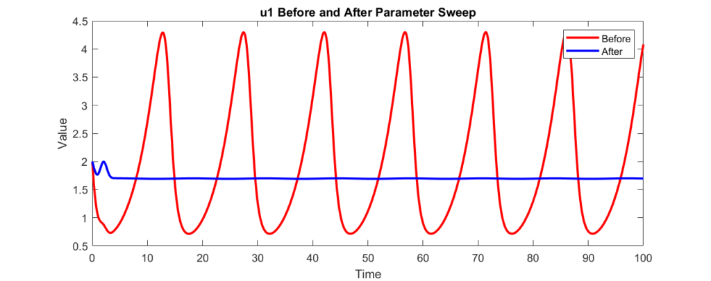
plot(sol0.Time, sol0.Solution(1,:), Color="r", LineWidth=2);
hold on
plot(sol.Time, sol.Solution(1,:), Color="b", LineWidth=2);
hold off
legend("Before", "After");
title("u1 Before and After Parameter Sweep");
xlabel("Time");
ylabel("Value");

Alright. So, here's the MATLAB workflow we're going to work with. In this case, it's fairly minimal. That's for demonstration purposes, but the main point is we have some workflow, but there's a particular part of the workflow that's causing us grief, and we want that to be faster, but we want to make it faster without entirely destroying or disrupting our workflow.

So, I'm going to start this running.

The Workflow

In this workflow, we have some pre-processing. We're just getting inputs ready for our computation. The core computation in this workflow is this gridsearch function. This gridsearch function is our implementation of that parameter sweep that I mentioned. And then once we have the output, we do some post-processing. In this case, we're just plotting values.

But again, the main point is that we have a workflow, but there's a pain point in that workflow that we want to be better. We want to make it better with Julia.

MATLAB Results

So there are our results. Alright, so here I'm plotting the first state variable before the parameter sweep and after the parameter sweep. And as expected, we see that the oscillations are smaller than before. And then if we look at the elapsed time, it took about 40 seconds for this to run in MATLAB.

Translating to Julia

Okay. So now we want Julia. So, the first step is to take the part of the workflow that we want to improve, and we're going to translate that into Julia.

# JuliaModel/src/gridsearch.jl

function gridsearch(
    u0::Vector{Float64},
    tspan::Vector{Float64},
    p::Vector{Float64},
    cb_times::Vector{Float64},
    cb_values::Vector{Float64},
    p_opt_indexes::Vector{Int64},
    grid_vals::NTuple{5, Vector{Float64}},
    lb_cons::Float64,
    ub_cons::Float64,
    abstol::Float64,
    reltol::Float64,
)

    # `p` is updated in place during the callbacks,
    # so take a copy that will be used to re-initialize `p`
    # at the start of each loop iteration below.
    p_original = copy(p)

    callback = get_callbacks(cb_times, cb_values)

    prob = ODEProblem{true}(dynamics!, u0, (tspan[1], tspan[2]), p)
    solver = DP5()

    sol0 = OrdinaryDiffEq.solve(prob, solver; callback, abstol, reltol)
    loss0 = max_variation(sol0)

    losses = Array{Float64, length(grid_vals)}(undef, length.(grid_vals)...)
    loss_opt = loss0
    p_opt = p_original[p_opt_indexes]
    for (i, p_vals) in enumerate(Iterators.product(grid_vals...))
        p .= p_original
        p[p_opt_indexes] .= p_vals
        new_prob = remake(prob; p)
        sol = OrdinaryDiffEq.solve(new_prob, solver; callback, abstol, reltol)
        if constraints_met(sol, lb_cons, ub_cons)
            l = max_variation(sol)
            if l < loss_opt
                loss_opt = l
                p_opt .= p_vals
            end
            losses[i] = l
        else
            losses[i] = Inf
        end
    end

    return (p_opt, loss_opt, loss0, losses)

end

So, we take the gridsearch function, we look at its implementation, we translate it into Julia, and we end up with a Julia function. I'm calling it gridsearch just like the MATLAB function. It takes the same inputs. It does the parameter sweep. It returns the same outputs as the MATLAB version. So the same computation, just now written in Julia instead of MATLAB.

And then we're going to house this function inside of a Julia package. In this case I called the Julia package JuliaModel. So now we have a Julia package. It has our Julia implementation of gridsearch, our parameter sweep.

Using MATFrost.jl

Now we need to build a bridge using MATFrost.jl. So, MATFrost.jl needs to be a dependency of our Julia package, even if the package doesn't use it at all, because what we're going to do is instantiate our Julia package's package environment. Then import MATFrost.jl and then call MATFrost.install. And what this does is it takes our Julia package and creates a MATLAB class out of that package, and in this case and it uses the same name.

So now we have a JuliaModel Julia package, but now we have a JuliaModel MATLAB class, which we'll use to interface with Julia. So this is what MATFrost.jl created for us.

Minimizing Disruptions

So now that we have that MATLAB class, now we need to start using this code to start interfacing with Julia. Now, we could add this directly to the workflow itself, but again, we want to minimize disruptions to the workflow, especially if we have colleagues that are also working on this workflow simultaneously with us.

So, the key idea here is we want calling out to Julia to be an implementation detail from the perspective of the workflow. So we don't want the workflow to care that we're calling out to Julia. We want the workflow to work as is.

So, what we're going to do is we're going to create a new MATLAB function, but within that function we call out to Julia. This MATLAB function I'm going to call gridsearch_julia, and importantly it needs the same API as whatever function we're replacing. So, I'm going to have it take the same inputs. It's going to return the same output, but then internally there's not much to it, again, because all the functionality is in Julia.

% gridsearch_julia.m

function [p_opt, loss_opt, loss0, losses] = gridsearch_julia(u0, tspan, p, p_opt_indexes, grid_vals, options)

    arguments

        u0
        tspan
        p
        p_opt_indexes
        grid_vals
        options.lb_cons = 1.65
        options.ub_cons = 2.25
        options.abstol = 1e-7
        options.reltol = 1e-7

    end

    jl = get_julia();

    out = jl.gridsearch(u0, tspan, p.p, p.cb_times, p.cb_values, p_opt_indexes, grid_vals, ...
        options.lb_cons, options.ub_cons, options.abstol, options.reltol);

    [p_opt, loss_opt, loss0, losses] = out{:};

end

What this function is going to do is I have this function get_julia which is a function I wrote that instantiates a JuliaModel object. Then with that object I can interface with Julia. So if I do jl.gridsearch right here, this gridsearch is not the MATLAB function. This is the gridsearch that I wrote in Julia in my Julia package. So what we're doing here is taking our MATLAB values and passing them over to Julia. Julia is going to run the gridsearch function I defined in Julia. It'll do the parameter sweep and then it will return a Tuple of values which is a cell array in MATLAB. So I just unpack that cell array to get the appropriate output for this function.

But again the main point to minimize disruption for the workflow is that this new function needs to have the same API so that from the workflow's perspective nothing changes.

Julia-MATLAB Results

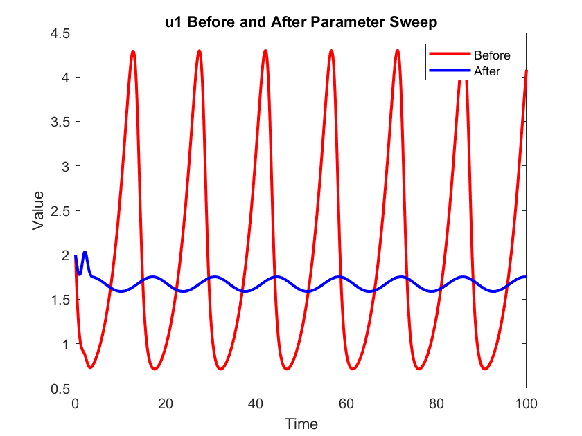
Let's see how this works. So, I'm just going to change the one function. (Change gridsearch to gridsearch_julia in demo.m.) Importantly I'm not changing any of the pre-processing or post-processing. I'm not changing any of the inputs or outputs. And then if I run it I get my result. The plot looks pretty much the same as last time, maybe exactly the same. And if we look at the timing, it was 100 times faster.

So, from the workflow's perspective, essentially nothing changed. I called out to a new function, but didn't have to change any the pre- or post-processing, but now the workflow runs 100 times faster than before.

So this was a 40-second version of the parameter sweep, not the five hour version. So, does it scale? Let's look at some other benchmarks.

ODE Solve Timing: MATLAB vs Julia-MATLAB

Alright, first looking at a single ODE solve. If we just did a single ODE solve in Julia and then did the Julia-MATLAB integration, that ODE solve takes 10 milliseconds. So, it's twice as fast as the pure MATLAB version. I will note that there is a significant overhead to using MATFrost.jl for the first call, but subsequent calls are faster. So a 2x speed up, that's something, but it's not the 10 to 1000 times speed up that we were seeing with the SciML benchmarks. But again, we don't typically solve an ODE a single time.

So what about the parameter sweep? You'll recall that in MATLAB the parameter sweep with 200,000 ODE solves took about five hours to run. In Julia, that time dropped to less than two minutes. So that's 163 times faster than the pure MATLAB version.

So I think that's fast enough for this meme. I am speed. Julia is speed. So that's amazing. We took our workflow, we created a new MATLAB function that called out to Julia internally (but from the workflow's perspective nothing really changed) but now it's 163 times faster.

Uncompromised Simulation Accuracy

Okay, so it's faster, but now the other question is are the results still good or are they garbage now.

The results are still good. Here, I'm plotting the first state variable before and after the parameter sweep; the MATLAB results are in red, the blue dots are the Julia results. And we see that the Julia results align with the MATLAB results.

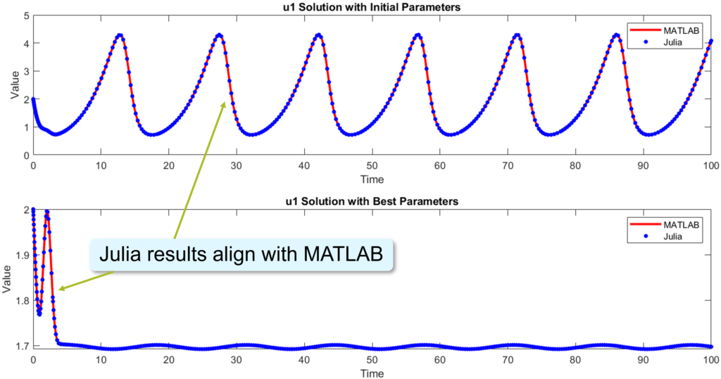
I also checked all the other state variables, and in all cases all of the Julia-MATLAB integrated results are within 1/100th of a percent compared to the MATLAB results. So, we achieve the accuracy that we want for our simulations at a fraction of the computational cost.

Julia-MATLAB Integration with GLCS

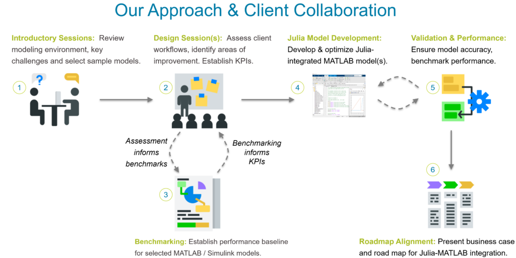
So now if you want these speed ups in your code, but you're not quite sure how to start, feel free to reach out to us at GLCS. We have an approach for helping clients pinpoint these areas of concern in their MATLAB workflows. We help translate the code to Julia and reintegrate it back into MATLAB and we ensure that we meet the accuracy and performance metrics that we need to.

Conclusion

So, unlock up to 100 times faster performance by integrating Julia. In today's example, we saw even faster than 100 times faster. Adopt Julia seamlessly. Integrate it step by step without disrupting your MATLAB workflows. So, enhance the MATLAB code that you have. Elevate its capabilities by integrating Julia and taking advantage of its speed and flexibility.

Thank you.

Q&A

1. Audience: Can you show us that get_julia function you mentioned?

   Yeah. So we want to see the get_julia function that I wrote in MATLAB. So yes, here it is. So basically I made use of a persistent variable to make sure I'm not reinitializing the Julia instance every time. So I'm reusing the same Julia instance every time I call this function. But the first time there's that overhead that I mentioned.

   Audience: Your MATLAB code isn't showing.

   function jl = get_julia()
   
       persistent jl_
       if isempty(jl_)
           mjl = JuliaModel();
           jl_ = mjl.JuliaModel;
       end
   
       jl = jl_;
   
   end
   

   Oh, thank you. I need to actually get me out of the slideshow. There we go. Okay. Persistent variable. So that way on subsequent calls to the function, I'm using the same initialization of the Julia runtime. So we're not wasting resources every time. But yeah, here is where we're actually initializing the JuliaModel MATLAB object. Yeah, there's nothing to it. There's no parameters to—I mean you can change the Julia version if you want but if you have everything set up in your PATH you don't need to pass anything to it.

2. Audience: Just a quick question, about how long did it take to, when you call MATFrost.jl to install JuliaModel, how long does that take?

   That's a good question. I don't remember off the top of my head.

   Audience: Well, it was quick, I'm assuming, or it just builds a little bit of MATLAB code, right?

   Right, if I remember correctly, it was on order of seconds, maybe minutes, but nothing terrible.

3. Audience: Does MATFrost.jl work with Linux or is it still like only for Windows?

   As far as I know, it's only supported for Windows.

4. Audience: Some of these numbers scare me a little with the performance comparisons between Julia and MATLAB. I know there's a huge difference in LAPACK and BLAS versioning, right, MATLAB typically goes for a more numerical stable version of LAPACK versus if Julia will use OpenBLAS by default, I think (I might be wrong on that). Could you tell me what version of each you're using for both?

   I do not know what versions I'm using.

   Audience: You just, in the MATLAB terminal, just do version -lapack. There's an "i" in "version".

   Oh, thank you. Is it capital LAPACK or lower?

   Audience: That's correct. Yeah. Okay, that is a faster one. Okay.

5. Audience: Can you actually like create structs or more complicated types than arrays with this?

   So can you create structs and arrays in Julia, are you saying?

   Audience: No no, like in MATLAB can you like create structs from Julia? Like if you define a data type in Julia can you like create it here in MATLAB?

   Yeah. So one of the key things to working with MATFrost.jl is everything needs to be concretely typed. So, like, if you create a struct, you can have nested structs and they basically get translated to MATLAB structs, but you need to concretely type it as a Float64 or an Int depending on whatever data type you have. So, no abstract types, and the function calls also need to be typed.

6. Audience: I remember a long time ago when I was calling C code from MATLAB it had to use these MEX files. Is that what it's using under the hood here or is there some new fancier way of calling external code and MEX files that this is using?

   Yeah, so MATFrost.jl does use a MEX file to work.

Additional Links

• JuliaCon Talk Submission Page
  • Submission page for the talk, including an abstract and summary.
• Julia and MATLAB^® Integration at GLCS
  • Our web page detailing our Julia and MATLAB^® integration service.

MATLAB is a registered trademark of The MathWorks, Inc.

Cover image: The JuliaCon 2025 logo was obtained from https://juliacon.org/2025/.