
MRI Scan Simulation Made Easy with BlochSim.jl
Learn how to simulate the signal acquired from an MRI scan.
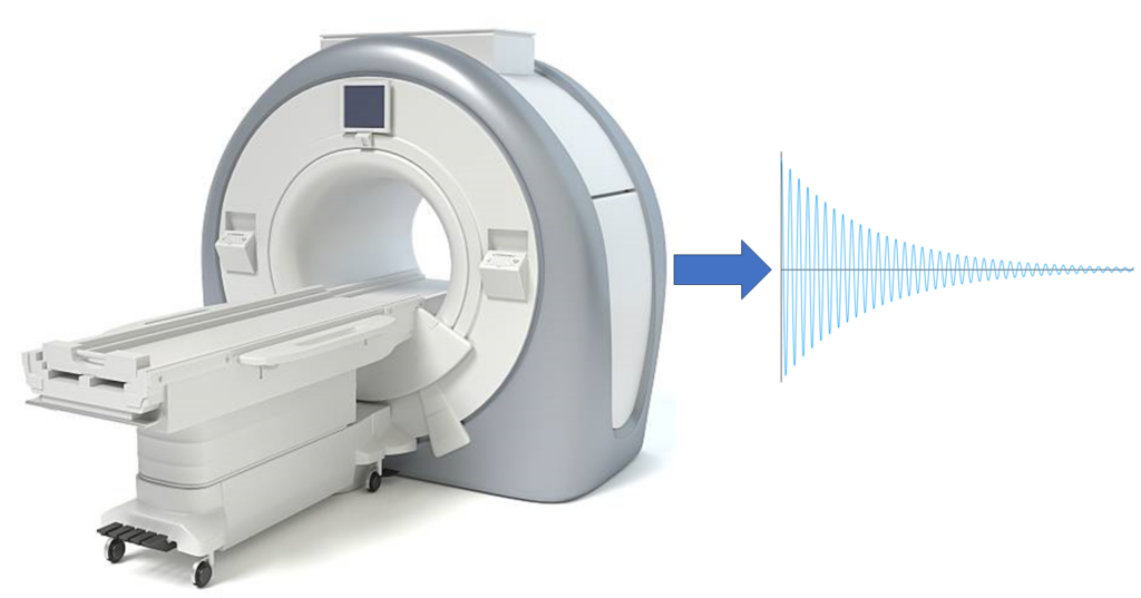
MRI scans manipulate magnetization vectors to produce an observable signal.
Often it can be useful to simulate what signal an MRI scan will generate. Example scenarios include simulating MRI signals for educational purposes, for developing a new MRI scan, or for fitting model parameters to an acquired signal.
In this post, we will learn how to use the Julia programming language, a free and open source programming language that excels especially in scientific computing, to simulate the signal generated by an MRI scan. Specifically, we will use the BlochSim.jl package to simulate a balanced steady-state free precession (bSSFP) scan.
Note that this post assumes a basic understanding of MRI pulse sequences and Bloch simulations. See our previous posts for an overview of the Bloch equations and an overview of BlochSim.jl.
Prerequisites
To run the code in this post, both Julia and BlochSim.jl need to be installed. See our previous post for installation instructions.
bSSFP
First, we need to review bSSFP so we know how to simulate it.
Here is a pulse sequence diagram of bSSFP (source).
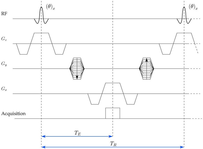
For this post, we are not simulating signal localization, so we will ignore the imaging gradients.
Thus, for each TR we will simulate
- excitation,
- free precession until the echo time, and
- free precession until the end of the TR.
This, by itself, would be essentially the same simulation as done in our previous post. However, two aspects of bSSFP make simulating it a bit more interesting.
- bSSFP, as the name states, is a steady-state scan. This means we don’t simulate just one excitation followed by free precession to the echo time. Instead, we need to simulate multiple TRs until we get to steady-state. We can do this either by manually simulating multiple TRs or by mathematically computing the steady-state magnetization. More on this later.
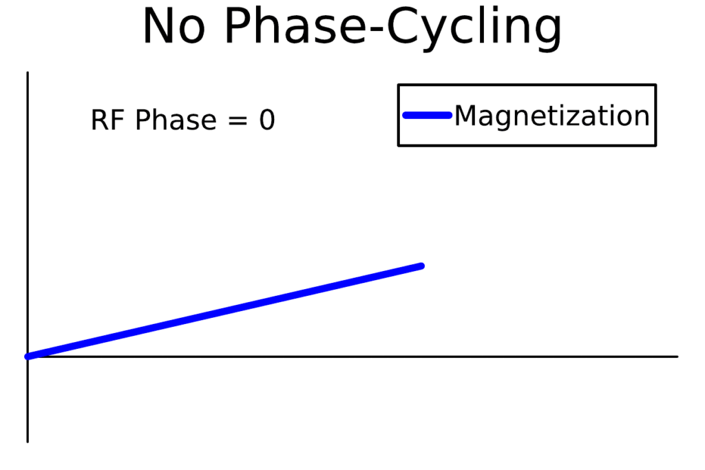
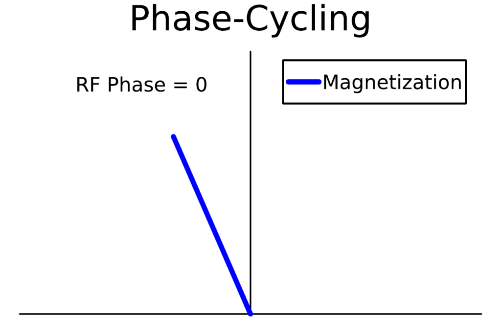
- bSSFP utilizes phase-cycling, where the phase of the RF pulse is incremented after each TR.
Therefore,
our goal is to write a Julia function
(that we will call bssfp)
that computes the steady-state signal
given by a bSSFP scan
that uses phase-cycling.
Throughout this post,
we will be editing
a text file called bssfp.jl
that will load BlochSim.jl
and define our bssfp function.
Function Outline
We will begin
with an outline
of what our bssfp function needs to do.
# bssfp.jl

using BlochSim

# Step 0: Specify the inputs to the function.
function bssfp(inputs)

    # Step 1: Create a `Spin` object.
    # Step 2: Create the RF pulse.
    # Step 3: Compute the steady-state signal.

end
First,
we need to specify
what inputs bssfp needs.
We need values for M0, T1, T2, and off-resonance frequency \( \Delta f \)
to create a Spin object,
a flip angle \( \alpha \)
to create the RF pulse,
and the TR, TE, and phase-cycling factor \( \Delta\phi \) to use.
We will also add an input
that specifies how to compute
the steady-state magnetization.
# bssfp.jl

using BlochSim

function bssfp(M0, T1, T2, Δf, α, TR, TE, Δϕ, manual_ss = false)

    # Step 1: Create a `Spin` object.
    # Step 2: Create the RF pulse.
    # Step 3: Compute the steady-state signal.

end
Here we see that Julia allows
using Greek letters in variable names,
which helps the code look more like the math,
enhancing readability.
(To type, e.g., α,
type \alpha and then press TAB,
and similarly for other Greek letters.)
We also made manual_ss an optional argument.
If the user does not specify manual_ss,
it will default to false.
Now we can focus on writing code for each step outlined above.
Step 1: Create a Spin Object
As discussed in our previous post,
a Spin object is created as follows.
spin = Spin(M0, T1, T2, Δf)
That’s it!
So let’s update bssfp.
# bssfp.jl

using BlochSim

function bssfp(M0, T1, T2, Δf, α, TR, TE, Δϕ, manual_ss = false)

    # Step 1: Create a `Spin` object.
    spin = Spin(M0, T1, T2, Δf)

    # Step 2: Create the RF pulse.
    # Step 3: Compute the steady-state signal.

end
Step 2: Create the RF Pulse
In this simulation,
we will assume the excitation pulse
is very short
relative to relaxation and off-resonance effects.
In this case,
we will use an InstantaneousRF object
for the RF pulse
that will simulate excitation
by just rotating the magnetization vector.
rf = InstantaneousRF(α)
Let’s add that to bssfp.
# bssfp.jl

using BlochSim

function bssfp(M0, T1, T2, Δf, α, TR, TE, Δϕ, manual_ss = false)

    # Step 1: Create a `Spin` object.
    spin = Spin(M0, T1, T2, Δf)

    # Step 2: Create the RF pulse.
    rf = InstantaneousRF(α)

    # Step 3: Compute the steady-state signal.

end
Step 3: Compute the Steady-State Signal
Now we are ready to tackle the core of the simulation. As mentioned earlier, there are two ways to go about computing the steady-state signal:
- we can manually simulate multiple TRs, or
- we can mathematically compute the steady-state magnetization.
We will discuss how to do both.
Version 1: Simulate Multiple TRs
The idea behind simulating multiple TRs is to simulate for long enough so that the magnetization reaches a steady-state. A good rule of thumb is to simulate for a few T1’s worth of time. Thus, the number of TRs we will simulate is 3T1 / TR, rounded up so we get an integer value.
nTR = ceil(Int, 3 * T1 / TR)
(Of course, the longer we simulate the closer to the true steady-state we will get.)
Then for each TR,
we have excitation followed by free precession.
But we also need to remember
to increment the phase of the RF pulse.
That means we will need to create
a new InstantaneousRF object
for each excitation.
In this case,
we will pass in the flip angle
as we did previously,
but we will also pass in the phase of the RF pulse
(which will be the phase of the previous pulse
plus the phase-cycling increment).
for i = 1:nTR
    excite!(spin, rf)
    freeprecess!(spin, TR)
    rf = InstantaneousRF(α, rf.θ + Δϕ)
end
Now we have the magnetization at the end of the TR, but we want the signal at the echo time. So we need to excite one more time, and then free precess until the echo time.
excite!(spin, rf)
freeprecess!(spin, TE)
Then the steady-state signal can be obtained. One detail to remember, however, is that when doing phase-cycling, the phase of the receiver coil is matched to the phase of the RF pulse. To simulate this, we will multiply our signal by a phase factor.
sig = signal(spin) * cis(-rf.θ)
(cis(θ) is an efficient way
to compute \( e^{i \theta} \).)
And there we have our steady-state signal!
Let’s update bssfp.
# bssfp.jl

using BlochSim

function bssfp(M0, T1, T2, Δf, α, TR, TE, Δϕ, manual_ss = false)

    # Step 1: Create a `Spin` object.
    spin = Spin(M0, T1, T2, Δf)

    # Step 2: Create the RF pulse.
    rf = InstantaneousRF(α)

    # Step 3: Compute the steady-state signal.
    if manual_ss
        # Version 1: Simulate multiple TRs.
        nTR = ceil(Int, 3 * T1 / TR)
        for i = 1:nTR
            excite!(spin, rf)
            freeprecess!(spin, TR)
            rf = InstantaneousRF(α, rf.θ + Δϕ)
        end
        excite!(spin, rf)
        freeprecess!(spin, TE)
        sig = signal(spin) * cis(-rf.θ)
    else
        # Version 2: Mathematically compute the steady-state.
        # This version is used by default if `manual_ss` is not provided.
    end

    return sig

end
Now let’s see how to compute the steady-state signal a different way.
Version 2: Mathematically Compute the Steady-State
In steady-state, a magnetization vector immediately after excitation (call it \( \mathbf{M}^{+} \)) is the same as the one immediately after the previous excitation (call it \( \mathbf{M} \)). Let \( \mathbf{A} \) and \( \mathbf{B} \) be such that \( \mathbf{A} \mathbf{M} + \mathbf{B} \) applies free precession to the magnetization vector, and let \( \mathbf{R} \) be the rotation matrix that represents the instantaneous excitation. Then in steady-state we have
Solving for \( \mathbf{M} \) gives us
where \( \mathbf{I} \) is the identity matrix.
This derivation assumes a constant RF phase,
so we need to account for phase-cycling somehow.
Phase-cycling in bSSFP shifts the off-resonance profile,
so it will suffice to use a Spin object
with a suitably chosen off-resonance frequency
to simulate phase-cycling.
Let’s use this derivation in our code.
spin_pc = Spin(M0, T1, T2, Δf - (Δϕ / 2π / (TR / 1000)))
(R,) = excite(spin_pc, rf)
(A, B) = freeprecess(spin_pc, TR)
M = (I - R * A) \ (R * B)
Here, I comes from the LinearAlgebra
standard library module,
so we will need to make sure
to load it.
Notice we didn’t modify spin,
so we need to make sure to copy
the computed steady-state magnetization
to spin.
copyto!(spin.M, M)
The above gives us the steady-state magnetization immediately after excitation, so now we need to simulate free precession until the echo time.
freeprecess!(spin, TE)
Then we can get the steady-state signal.
sig = signal(spin)
Updating bssfp gives us the following.
# bssfp.jl

using BlochSim, LinearAlgebra

function bssfp(M0, T1, T2, Δf, α, TR, TE, Δϕ, manual_ss = false)

    # Step 1: Create a `Spin` object.
    spin = Spin(M0, T1, T2, Δf)

    # Step 2: Create the RF pulse.
    rf = InstantaneousRF(α)

    # Step 3: Compute the steady-state signal.
    if manual_ss
        # Version 1: Simulate multiple TRs.
        nTR = ceil(Int, 3 * T1 / TR)
        for i = 1:nTR
            excite!(spin, rf)
            freeprecess!(spin, TR)
            rf = InstantaneousRF(α, rf.θ + Δϕ)
        end
        excite!(spin, rf)
        freeprecess!(spin, TE)
        sig = signal(spin) * cis(-rf.θ)
    else
        # Version 2: Mathematically compute the steady-state.
        # This version is used by default if `manual_ss` is not provided.
        spin_pc = Spin(M0, T1, T2, Δf - (Δϕ / 2π / (TR / 1000)))
        (R,) = excite(spin_pc, rf)
        (A, B) = freeprecess(spin_pc, TR)
        M = (I - R * A) \ (R * B)
        copyto!(spin.M, M)
        freeprecess!(spin, TE)
        sig = signal(spin)
    end

    return sig

end
Now bssfp is complete
and ready to use!
Using bssfp
To use bssfp,
we need to run the bssfp.jl file
that loads BlochSim.jl
and defines bssfp.
julia> include("bssfp.jl")
bssfp (generic function with 2 methods)
First, let’s make sure the two methods for computing the steady-state magnetization give approximately the same result.
julia> (M0, T1, T2, Δf, α, TR, TE, Δϕ) = (1, 1000, 80, 0, π/6, 5, 2.5, π/2)
(1, 1000, 80, 0, 0.5235987755982988, 5, 2.5, 1.5707963267948966)

julia> sig_manual = bssfp(M0, T1, T2, Δf, α, TR, TE, Δϕ, true)
0.09889476203144602 + 0.09290409266118088im

julia> sig_exact = bssfp(M0, T1, T2, Δf, α, TR, TE, Δϕ)
0.09880282817239999 + 0.09281666742806782im

julia> isapprox(sig_exact, sig_manual; rtol = 0.001)
true
The results are less than 0.1% different from each other, indicating the manually simulated steady-state does approach the mathematically computed steady-state, as expected.
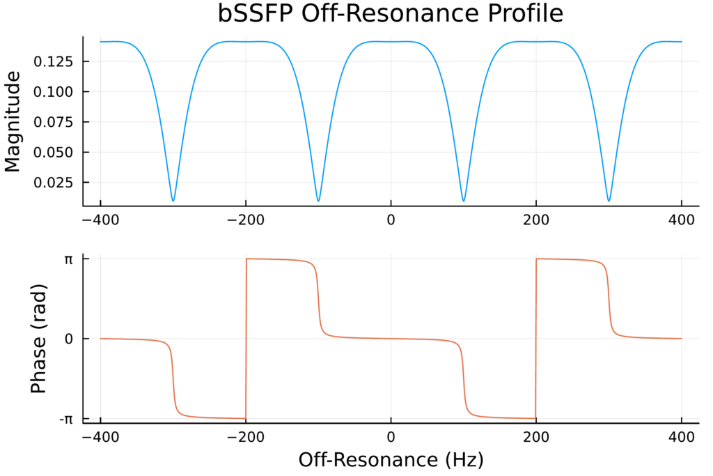
Now let’s use bssfp
to plot the characteristic bSSFP off-resonance profile.
First we compute the steady-state signal
for various off-resonance values.
julia> (M0, T1, T2, α, TR, TE, Δϕ, N) = (1, 1000, 80, π/6, 5, 2.5, π, 801)
(1, 1000, 80, 0.5235987755982988, 5, 2.5, π, 801)

julia> Δf = range(-2 / (TR / 1000), 2 / (TR / 1000), N)
-400.0:1.0:400.0

julia> sig = bssfp.(M0, T1, T2, Δf, α, TR, TE, Δϕ);
Note the dot (.) when calling bssfp.
This essentially is shorthand for
sig = zeros(ComplexF64, length(Δf))
for i = 1:length(Δf)
    sig[i] = bssfp(M0, T1, T2, Δf[i], α, TR, TE, Δϕ)
end
(See our blog post on broadcasting for more information.)
And now we can plot the results.
julia> using Plots

julia> pmag = plot(Δf, abs.(sig); label = "", ylabel = "Magnitude", color = 1);

julia> pphase = plot(Δf, angle.(sig); label = "", xlabel = "Off-Resonance (Hz)", ylabel = "Phase (rad)", yticks = ([-π, 0, π], ["-π", "0", "π"]), color = 2);

julia> plot(pmag, pphase; layout = (2, 1))
Summary
In this post,
we have learned how to use BlochSim.jl
to simulate the steady-state signal
obtained from a bSSFP scan.
We used the bssfp function we wrote
to plot the characteristic bSSFP off-resonance profile
to demonstrate that our code produces the expected results.
Additional Links
- BlochSim.jl: A Julia Package for MRI Bloch Simulations
- Overview of BlochSim.jl and how to use it for a basic Bloch simulation.
- Simulating MRI Physics with the Bloch Equations
- Overview of the Bloch equations and how to write your own Bloch simulation code in Julia.
- BlochSim.jl
- Provides
MESEBlochSimandSPGRBlochSimobjects that simulate multi-echo spin echo (MESE) and spoiled gradient recalled echo (SPGR) scans, respectively.
- Provides
- STFR.jl
- Unregistered Julia package that uses BlochSim.jl for simulating small-tip fast recovery (STFR) scans (a type of steady-state scan).