Simulating MRI Physics with the Bloch Equations
Learn how to run Bloch simulations in the Julia programming language.
MRI is an important imaging modality with impressive diagnostic capabilities.
The equations that specify the physics of how MRI works are called the Bloch equations.
People who study MRI use the Bloch equations to simulate MRI scans. These simulations are called Bloch simulations.
In this post, we will learn how to simulate MRI physics in the Julia programming language, a free and open source programming language that excels especially in scientific computing.
Note that this post assumes a basic understanding of the Bloch equations and MRI in general.
Installing Julia
You can head over to Julia’s website to download the language on your own computer, or you can try out Julia in your web browser first.
Notation
Here is the mathematical notation used in this post.
- \( \mathbf{M} = [M_x, M_y, M_z] \): Magnetization vector
- \( M_{xy} = M_x + i M_y \): Transverse magnetization (\( i = \sqrt{-1} \))
- \( \mathbf{M}_0 = [0, 0, M_0] \): Equilibrium magnetization vector
- \( M_0 \): Equilibrium magnetization
- \( T_1 \): T1 time constant
- \( T_2 \): T2 time constant
- \( \Delta\omega \): Off-resonance frequency
- \( \omega_{1,x} \): Rotational frequency due to the excitation RF field (along x)
- \( \omega_{1,y} \): Rotational frequency due to the excitation RF field (along y)
Bloch Equations
MRI scans manipulate magnetization vectors, and the Bloch equations explain the physics of how that happens. The system of ordinary differential equations (ODE) that make up the Bloch equations is as follows.
Normally in MRI, however, we make important assumptions that lead to closed-form solutions.
Excitation
One assumption is that the RF excitation pulses are fast (instantaneous) relative to all the other dynamics. This leads to
(For simplicity, we assume the excitation pulse is aligned with the x-axis.)
The solution to this ODE is rotation, i.e.,
where \( \alpha \) is the flip angle.
Julia Code: Excitation
To simulate excitation in Julia,
we need a magnetization vector
and a rotation matrix.
Let’s say we start with
\( \mathbf{M}(t_0^{-}) = [0, 0, 1] \),
i.e., magnetization along the z-axis.
In Julia,
we create a variable M
and assign it the value of [0, 0, 1].
Here’s how it looks in the Julia prompt (REPL):
julia> M = [0, 0, 1]
3-element Vector{Int64}:
 0
 0
 1
Next we need the rotation matrix. First, we specify the flip angle, and then we make the rotation matrix.
julia> alpha = π / 2 # To type π, type \pi<tab>
1.5707963267948966

julia> R = [0 0 0; 0 cos(alpha) sin(alpha); 0 -sin(alpha) cos(alpha)]
3x3 Matrix{Float64}:
 0.0   0.0          0.0
 0.0   6.12323e-17  1.0
 0.0  -1.0          6.12323e-17
(Note that the result of cos(alpha) is 6.12323e-17,
not 0.0,
because of floating point rounding errors,
i.e., a computer can’t exactly represent
\( \frac{\pi}{2} \).)
Finally, the excitation can be simulated by multiplying the magnetization by the rotation matrix.
julia> M_ex = R * M
3-element Vector{Float64}:
 0.0
 1.0
 6.123233995736766e-17
We started with magnetization along the z-axis, applied a 90° excitation pulse along the x-axis, and ended up with magnetization along the y-axis as expected.
We have officially simulated MRI physics!
But excitation is just part of the physics, so let’s move on to free precession.
Free Precession
Free precession is what occurs when the RF excitation pulse is turned off. In this case, the Bloch equations become
The solution to this ODE is free precession, which includes the effects of off-resonance precession, T1 recovery, and T2 decay.
Julia Code: Free Precession
To simulate free precession in Julia, we need a magnetization vector, and we need to specify some constants. Let’s say we start with \( \mathbf{M}(t_0) = [0, 1, 0] \), i.e., magnetization along the y-axis, and let’s use the following constant values:
- \( M_0 = 1 \)
- \( T_1 = 1 \) second
- \( T_2 = 0.1 \) seconds
- \( \Delta\omega = 25\pi \) rad/s
- \( t – t_0 = 0.01 \) seconds
We can create M
and variables for the constants
and equilibrium magnetization.
julia> M = [0, 1, 0]
3-element Vector{Int64}:
 0
 1
 0

julia> (M0, T1, T2, dw, dt) = (1, 1, 0.1, 25π, 0.01)
(1, 1, 0.1, 78.53981633974483, 0.01)

julia> M0_vec = [0, 0, M0]
3-element Vector{Int64}:
 0
 0
 1
Next we can create the \( \mathbf{E} \) and \( \mathbf{F} \) matrices from above.
julia> E = [exp(-dt/T2) 0 0; 0 exp(-dt/T2) 0; 0 0 exp(-dt/T1)]
3x3 Matrix{Float64}:
 0.904837  0.0       0.0
 0.0       0.904837  0.0
 0.0       0.0       0.99005

julia> phi = dw * dt; F = [cos(phi) sin(phi) 0; -sin(phi) cos(phi) 0; 0 0 1]
3x3 Matrix{Float64}:
  0.707107  0.707107  0.0
 -0.707107  0.707107  0.0
  0.0       0.0       1.0
Finally, the free precession can be simulated.
julia> M_fp = M0_vec + E * F * (M - M0_vec)
3-element Vector{Float64}:
 0.6398166741645539
 0.639816674164554
 0.009950166250831893
Awesome, now we can simulate excitation and free precession, two major building blocks of MRI physics!
We can use these building blocks to perform a more complete simulation of MRI physics.
A More Complete Simulation
Let’s simulate how a magnetization vector evolves over time.
We will simulate a 1 ms excitation pulse followed by 9 ms of free precession with a time step of 10 μs.
julia> (t_ex, t_fp, dt) = (0.001, 0.009, 0.00001)
(0.001, 0.009, 1.0e-5)

julia> t_total = t_ex + t_fp
0.009999999999999998
In this case, however, we don’t want to assume the excitation is instantaneous. Instead, we will split the RF pulse into segments of width \( \Delta t \). For each segment, we will
- simulate free precession for a duration of \( \Delta t / 2 \),
- simulate an instantaneous RF pulse whose flip angle is determined by the current value of the RF waveform, and
- again simulate free precession for a duration of \( \Delta t / 2 \).
Thus we can still use our building blocks while simulating a more accurate excitation.
We will want to plot the magnetization over time,
so we will need to store the magnetization vector
at each time step of the simulation.
We can create a Vector of Vectors
with enough pre-allocated storage for the simulation.
julia> nsteps = round(Int, t_total / dt)
1000

julia> M = Vector{Vector{Float64}}(undef, nsteps + 1)
1001-element Vector{Vector{Float64}}:
 #undef
 ⋮
 #undef
We also need to specify the RF pulse. We will make a sinc pulse that gives a flip angle of 90°.
julia> nrf = round(Int, t_ex / dt)
100

julia> rf = sinc.(range(-3, 3, nrf));
Above, range(-3, 3, nrf) creates nrf equally spaced points
from -3 to 3, inclusive.
And sinc is a scalar function,
so we broadcast it, or apply it elementwise,
by adding the dot (.) after the function name.
The flip angle is not correct,
so we need to scale rf.
julia> rf .*= π/2 / sum(rf);
Finally, let’s start with magnetization in equilibrium and specify the other constants.
julia> (M0, T1, T2, dw) = (1, 1, 0.1, 25π)
(1, 1, 0.1, 78.53981633974483)

julia> M[1] = [0, 0, M0]
3-element Vector{Int64}:
 0
 0
 1
To aid with the simulation, we will make a function to do excitation and another to do free precession.
julia> function excite(M, alpha, M0, T1, T2, dw, dt)

           M_next = freeprecess(M, M0, T1, T2, dw, dt/2)
           R = [0 0 0; 0 cos(alpha) sin(alpha); 0 -sin(alpha) cos(alpha)]
           M_next = R * M_next
           M_next = freeprecess(M_next, M0, T1, T2, dw, dt/2)

           return M_next

       end
excite (generic function with 1 method)

julia> function freeprecess(M, M0, T1, T2, dw, dt)

           M0_vec = [0, 0, M0]
           E = [exp(-dt/T2) 0 0; 0 exp(-dt/T2) 0; 0 0 exp(-dt/T1)]
           phi = dw * dt
           F = [cos(phi) sin(phi) 0; -sin(phi) cos(phi) 0; 0 0 1]
           M_next = M0_vec + E * F * (M - M0_vec)

           return M_next

       end
freeprecess (generic function with 1 method)
Now we can run the simulation.
julia> for i = 1:nsteps
           if i <= nrf
               M[i+1] = excite(M[i], rf[i], M0, T1, T2, dw, dt)
           else
               M[i+1] = freeprecess(M[i], M0, T1, T2, dw, dt)
           end
       end
And with that, we have successfully simulated a realistic excitation pulse followed by free precession.
Now we want to visualize the results.
Simulation Results
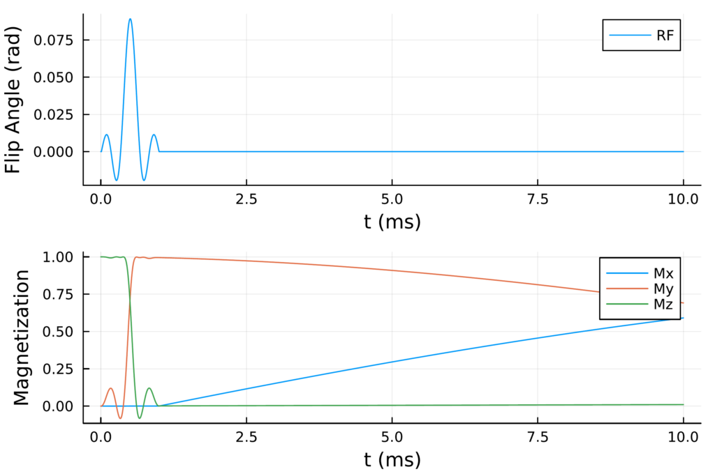
To plot the results, we will use the Plots.jl package. Our plot will have two subplots. The first will show the RF waveform, and the second will show \( M_x \), \( M_y \), and \( M_z \).
julia> using Plots

julia> t = (0:nsteps) .* (dt * 1000)
0.0:0.01:10.0

julia> rf = [0; rf; zeros(nsteps - nrf)];

julia> prf = plot(t, rf; label = "RF", xlabel = "t (ms)", ylabel = "Flip Angle (rad)");

julia> Mx = getindex.(M, 1); My = getindex.(M, 2); Mz = getindex.(M, 3);

julia> pM = plot(t, Mx; label = "Mx", xlabel = "t (ms)", ylabel = "Magnetization");

julia> plot!(pM, t, My; label = "My");

julia> plot!(pM, t, Mz; label = "Mz");

julia> plot(prf, pM; layout = (2, 1))
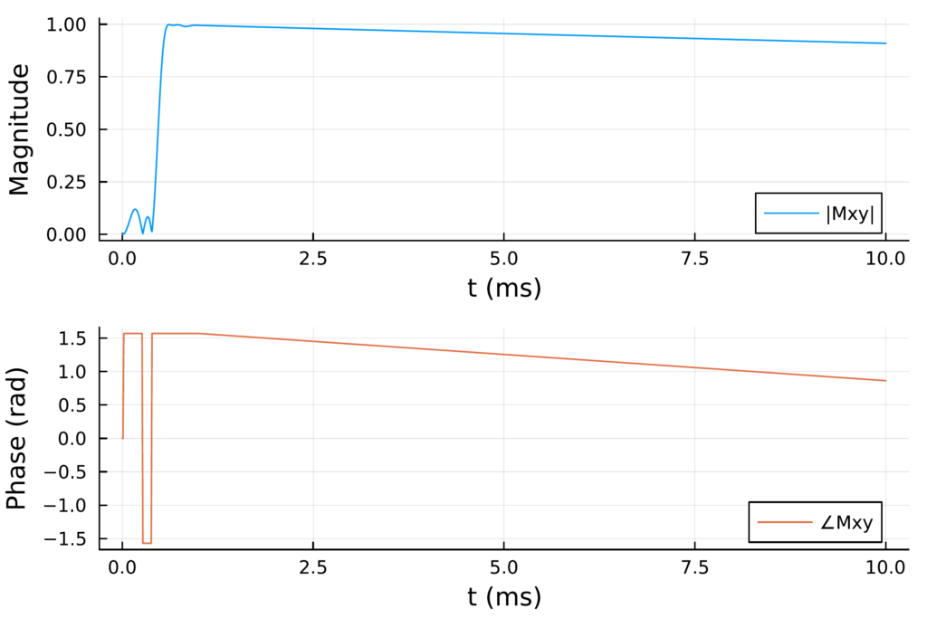
We can also plot the magnitude and phase of the transverse component of the magnetization (i.e., \( M_{xy} = M_x + i M_y \)).
julia> Mxy = complex.(Mx, My);

julia> pmag = plot(t, abs.(Mxy); label = "|Mxy|", xlabel = "t (ms)", ylabel = "Magnitude", color = 1);

# To type ∠, type \angle<tab>
julia> pphase = plot(t, angle.(Mxy); label = "∠Mxy", xlabel = "t (ms)", ylabel = "Phase (rad)", color = 2);

julia> plot(pmag, pphase; layout = (2, 1))
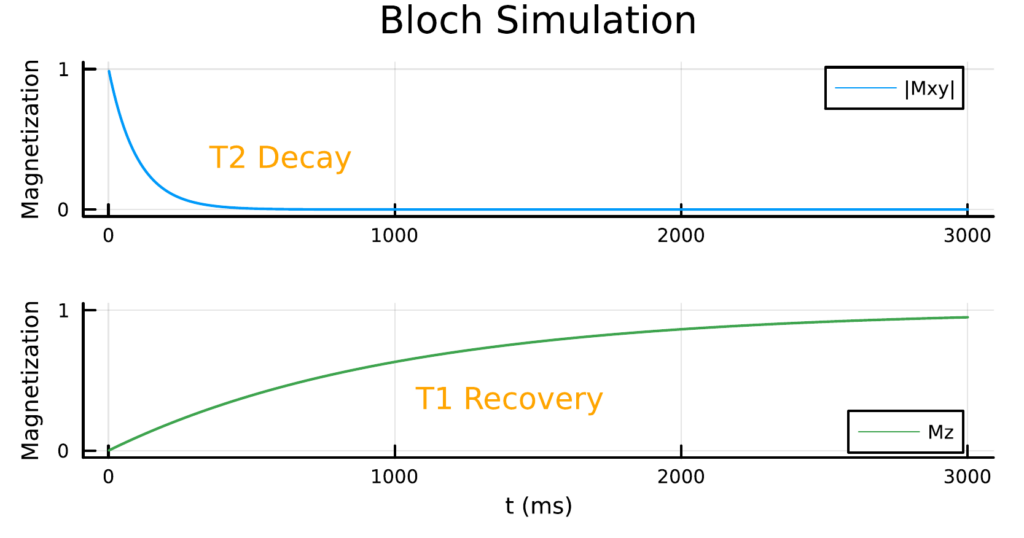
Finally,
if we want to see the magnetization recover to (almost) equilibrium,
we can increase t_fp (the free precession duration)
to, say, 3 * T1.
To reduce the number of time steps,
it is advisable to use a larger time step
for free precession than for excitation
(the results below used a 1 ms time step for free precession).
And now we can easily see the characteristic T2 decay, off-resonance precession, and T1 recovery of the magnetization vector, indicating we have done a successful Bloch simulation!
Summary
In this post, we have reviewed the Bloch equations and seen how to implement excitation and free precession in Julia. We have also seen how to run a Bloch simulation that tracks a magnetization vector over time, starting with an excitation pulse and continuing with free precession.
Additional Links
- BlochSim.jl
- Julia package for running Bloch simulations.
- BlochSim.jl: A Julia Package for MRI Bloch Simulations
- Blog post covering how to use BlochSim.jl.
- Simulating MRI Scans with BlochSim.jl
- Blog post covering a more in-depth use case for BlochSim.jl; specifically, simulating the signal acquired from a balanced steady-state free precession (bSSFP) scan.