Mastering MRI Bloch Simulations with BlochSim.jl in Julia
Learn how to use BlochSim.jl to run Bloch simulations.
Julia is a relatively new programming language that excels especially in scientific computing.
In addition to the functionality provided by the language itself, Julia boasts a large and growing collection of packages that can be seamlessly installed and loaded and that provide even more functionality.
In this post, we will learn how to use BlochSim.jl, a Julia package that provides functionality for running MRI Bloch simulations.
Note that this post assumes a basic understanding of the Bloch equations and MRI in general. See our previous post for a very brief overview of the Bloch equations (and a walkthrough of how to write your own Bloch simulation code in Julia).
Installing Julia
You can head over to Julia’s website to download the language on your own computer, or you can try out Julia in your web browser first.
Installing and Loading BlochSim.jl
We need to install BlochSim.jl. We can do so by running the following from the Julia prompt (also known as the REPL):
julia> using Pkg; Pkg.add("BlochSim")
Then we can load BlochSim.jl into our current Julia session.
julia> using BlochSim
Great, BlochSim.jl is installed and loaded, so now we can start learning how to use it!
The Bloch equations manipulate magnetization vectors, so first we will learn how BlochSim.jl represents a magnetization vector.
Spin: Representing a Magnetization Vector
BlochSim.jl uses Spins
to represent magnetization vectors.
More accurately,
a Spin represents an isochromat,
i.e., a magnetization vector
with associated values
for M0, T1, T2, and off-resonance frequency.
Thus, to construct a Spin,
we need to pass those values to the constructor.
julia> (M0, T1, T2, df) = (1, 1000, 80, 100)
(1, 1000, 80, 100)

julia> spin = Spin(M0, T1, T2, df)
Spin{Float64}:
 M = Magnetization(0.0, 0.0, 1.0)
 M0 = 1.0
 T1 = 1000.0 ms
 T2 = 80.0 ms
 Δf = 100.0 Hz
 pos = Position(0.0, 0.0, 0.0) cm
Some notes:
spin.Mis the magnetization vector associated with the isochromat. This vector is what will be manipulated by the Bloch equations.spin.Mby default starts in thermal equilibrium.- We can grab the x-component of the magnetization
with
spin.M.xorgetproperty(spin.M, :x)(similarly for y and z). - T1 and T2 are given in units of ms, while off-resonance uses Hz.
- The spin optionally can be given a position (useful if simulating B0 gradients).
Now that we have a spin, we can manipulate it with the Bloch equations.
Running a Bloch Simulation
We will simulate a 1 ms excitation pulse followed by 9 ms of free precession with a time step of 10 μs.
julia> (t_ex, t_fp, dt) = (1, 9, 0.01)
(1, 9, 0.01)

julia> t_total = t_ex + t_fp
10
We will want to plot the magnetization over time,
so we will need to store the magnetization vector
at each time step of the simulation.
We can create a Vector of Magnetizations
with enough pre-allocated storage for the simulation.
julia> nsteps = round(Int, t_total / dt)
1000

julia> M = Vector{Magnetization{Float64}}(undef, nsteps + 1)
1001-element Vector{Magnetization{Float64}}:
 #undef
 ⋮
 #undef
RF: Representing an RF Excitation Pulse
BlochSim.jl represents excitation pulses
with the RF object.
The constructor takes in the RF waveform
(in units of Gauss)
and the time step (in ms) to use
(and optionally a phase offset
and/or a B0 gradient).
For the excitation pulse, we will use a sinc pulse that gives a flip angle of 90°. First we will specify the shape.
julia> nrf = round(Int, t_ex / dt)
100

julia> waveform = sinc.(range(-3, 3, nrf));
(Note the dot (.) when calling sinc.
This calls sinc, a scalar function,
on each element of the input array.
See our blog post on broadcasting
for more information.)
And now we need to scale our waveform to get the desired flip angle.
julia> flip = π/2
1.5707963267948966

julia> waveform .*= flip / sum(waveform) / (GAMMA * dt / 1000);
Now that we have our waveform
we can construct an RF object.
julia> rf_full = RF(waveform, dt)
RF{Float64,Gradient{Int64}}:
 α = [0.0, 0.001830277817402092 … 0.001830277817402092, 0.0] rad
 θ = [0.0, 0.0 … 0.0, 0.0] rad
 Δt = 0.01 ms
 Δθ (initial) = 0.0 rad
 Δθ (current) = 0.0 rad
 grad = Gradient(0, 0, 0) G/cm
Using this RF object
would give us the magnetization vector
at the end of excitation,
but wouldn’t allow us to plot the magnetization
during excitation.
So instead,
we will pretend we have nrf separate excitations.
julia> rf = [RF([x], dt) for x in waveform]
100-element Vector{RF{Float64, Gradient{Int64}}}:
 RF([0.0], [0.0], 0.01, 0.0, Gradient(0, 0, 0))
 RF([0.001830277817402092], [0.0], 0.01, 0.0, Gradient(0, 0, 0))
 ⋮
 RF([0.0], [0.0], 0.01, 0.0, Gradient(0, 0, 0))
(Note that above we used a comprehension.)
excite and freeprecess
BlochSim.jl provides two main Bloch simulation functions:
excite for simulating excitation
and freeprecess for simulating free precession.
They each return a matrix A and a vector B
such that A * M + B applies the dynamics
to a magnetization vector M.
We will use these functions in our simulation.
julia> M[1] = copy(spin.M);

julia> for i = 1:nsteps
           if i <= nrf
               (A, B) = excite(spin, rf[i])
           else
               (A, B) = freeprecess(spin, dt)
           end
           M[i+1] = A * M[i] + B
       end
(Note that if we used M[1] = spin.M above,
i.e., without copying,
any modifications to spin.M
would also change M[1],
and vice versa,
because they both would refer
to the same computer memory location.)
And with that, we have successfully run a Bloch simulation!
Now we want to visualize the results.
Simulation Results
To plot the results, we will use the Plots.jl package, installed via
julia> using Pkg; Pkg.add("Plots")
Our plot will have two subplots. The first will show the RF waveform, and the second will show the x-, y-, and z-components of the magnetization vector over time.
julia> using Plots

julia> t = (0:nsteps) .* dt
0.0:0.01:10.0

julia> rf_plot = [0; waveform; zeros(nsteps - nrf)];

julia> prf = plot(t, rf_plot; label = "RF", xlabel = "t (ms)", ylabel = "Amplitude (G)");

julia> Mx = getproperty.(M, :x); My = getproperty.(M, :y); Mz = getproperty.(M, :z);

julia> pM = plot(t, Mx; label = "Mx", xlabel = "t (ms)", ylabel = "Magnetization");

julia> plot!(pM, t, My; label = "My");

julia> plot!(pM, t, Mz; label = "Mz");

julia> plot(prf, pM; layout = (2, 1))
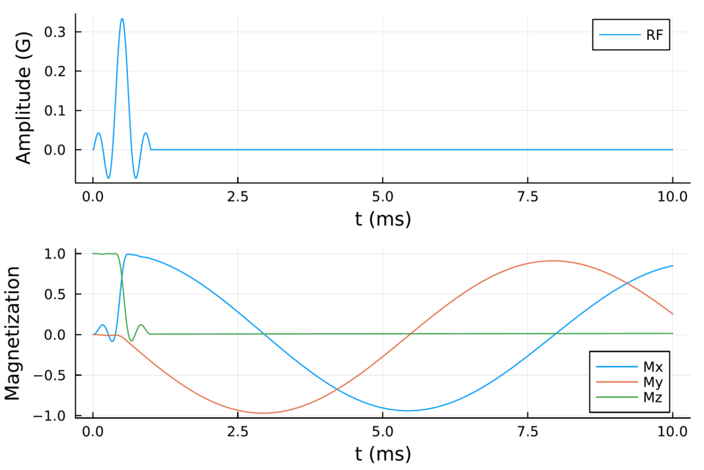
And there you have it! We can see the excitation occur followed by off-resonance precession. If we simulated free precession for longer we would also see T1 recovery and T2 decay.
Running a Bloch Simulation Without Plotting
But what if you don’t want to plot because you only care about the magnetization at the end of the simulation?
BlochSim.jl was made with this use case in mind.
Let’s repeat the Bloch simulation above, but this time we want only the magnetization at the end of the simulation.
We will reuse the following variables:
spin(Spinobject with the initial magnetization vector and tissue parameters)t_fp(free precession duration)rf_full(RFobject of duration 1 ms with a time step of 10 μs and a flip angle of 90°)
Since we don’t need to store intermediate magnetization vectors,
we can operate directly on spin.M,
reusing it instead of creating new Magnetization objects.
To do this,
we will use the functions excite! and freeprecess!.
Note the ! at the end of the above function names;
this is the Julia convention
for indicating a function mutates, or modifies,
one or more of its inputs
(typically the first input).
The functions excite! and freeprecess!
take the same inputs as their non-mutating counterparts.
But instead of returning a matrix A and a vector B,
they modify spin.M directly.
Also, since we aren’t storing intermediate magnetization vectors,
instead of looping for nsteps steps,
we call excite! and freeprecess!
just one time each.
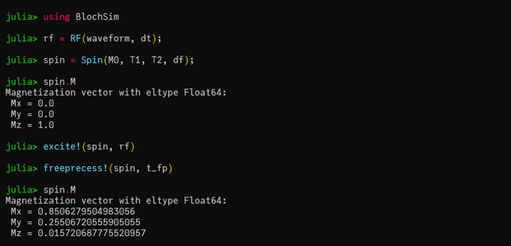
julia> excite!(spin, rf_full)

julia> freeprecess!(spin, t_fp)
Now spin.M is the magnetization
at the end of the Bloch simulation.
julia> spin.M
Magnetization vector with eltype Float64:
 Mx = 0.8506279504983056
 My = 0.25506720555905055
 Mz = 0.015720687775520957
And if we want the complex-valued MRI signal,
we just use the signal function.
julia> signal(spin)
0.8506279504983056 + 0.25506720555905055im
We can also verify that the two approaches give the same result (up to floating point rounding errors) at the end of the simulation.
julia> M[end] ≈ spin.M # To type ≈, type \approx<tab>
true
So now we can run Bloch simulations in two ways:
- where we keep track of the intermediate magnetization vectors for plotting purposes, and
- where we call
excite!andfreeprecess!one time each to compute the magnetization only at the end of the simulation.
Summary
In this post,
we have seen
how to use BlochSim.jl
to run Bloch simulations.
In particular,
we learned how to construct a Spin object
and an RF object,
and we manipulated magnetization vectors
using excite/excite! and freeprecession/freeprecession!.
Additional Notes about BlochSim.jl
excite!andfreeprecess!could have been used in the plotting version of the Bloch simulation. Then, instead ofM[i+1] = A * M[i] + B, we would needM[i+1] = copy(spin.M).InstantaneousRFcan be used in place ofRFif one wants to assume the RF pulse is very fast compared to T1/T2/off-resonance effects. (This is a typical assumption.)- For advanced MRI users/researchers:
BlochSim.jl provides a
SpinMCobject for simulating multiple compartments using the Bloch-McConnell equations.
Additional Links
- Simulating MRI Physics with the Bloch Equations
- Overview of the Bloch equations and how to write your own Bloch simulation code in Julia.
- Simulating MRI Scans with BlochSim.jl
- Blog post covering a more in-depth use case for BlochSim.jl; specifically, simulating the signal acquired from a balanced steady-state free precession (bSSFP) scan.
- BlochSim.jl’s documentation
- Documentation for the different functions and structs defined by BlochSim.jl.