Variables and functions are the building blocks of any programmer's code. Variables allow computations to be reused, and functions help keep code organized.

In this post, we will cover some of the basics of variables and functions in Julia, a relatively new, free, and open-source programming language. In particular, we will discuss what a variable is, what sorts of data can be assigned to a variable, and how to define and use functions.

Variables

A variable is a label used to refer to an object.

julia> a = 1
1

In the above code snippet, we assigned a value of 1 to a variable called a. Now we can use a in other expressions, and the value of a (1 in this case) will be used.

julia> a + 2
3

We can also reassign variables.

julia> a = 4
4

julia> a = "Hello"
"Hello"

julia> a = [1, 2, 3]
3-element Vector{Int64}:
 1
 2
 3

We can even use Unicode characters! We can write many math symbols by typing the corresponding LaTeX command and then pressing <tab>. Here, we assign π (a Julia constant equal to \( \pi \) and typed with \pi<tab>) to θ (typed with \theta<tab>).

julia> θ = π
π = 3.1415926535897...

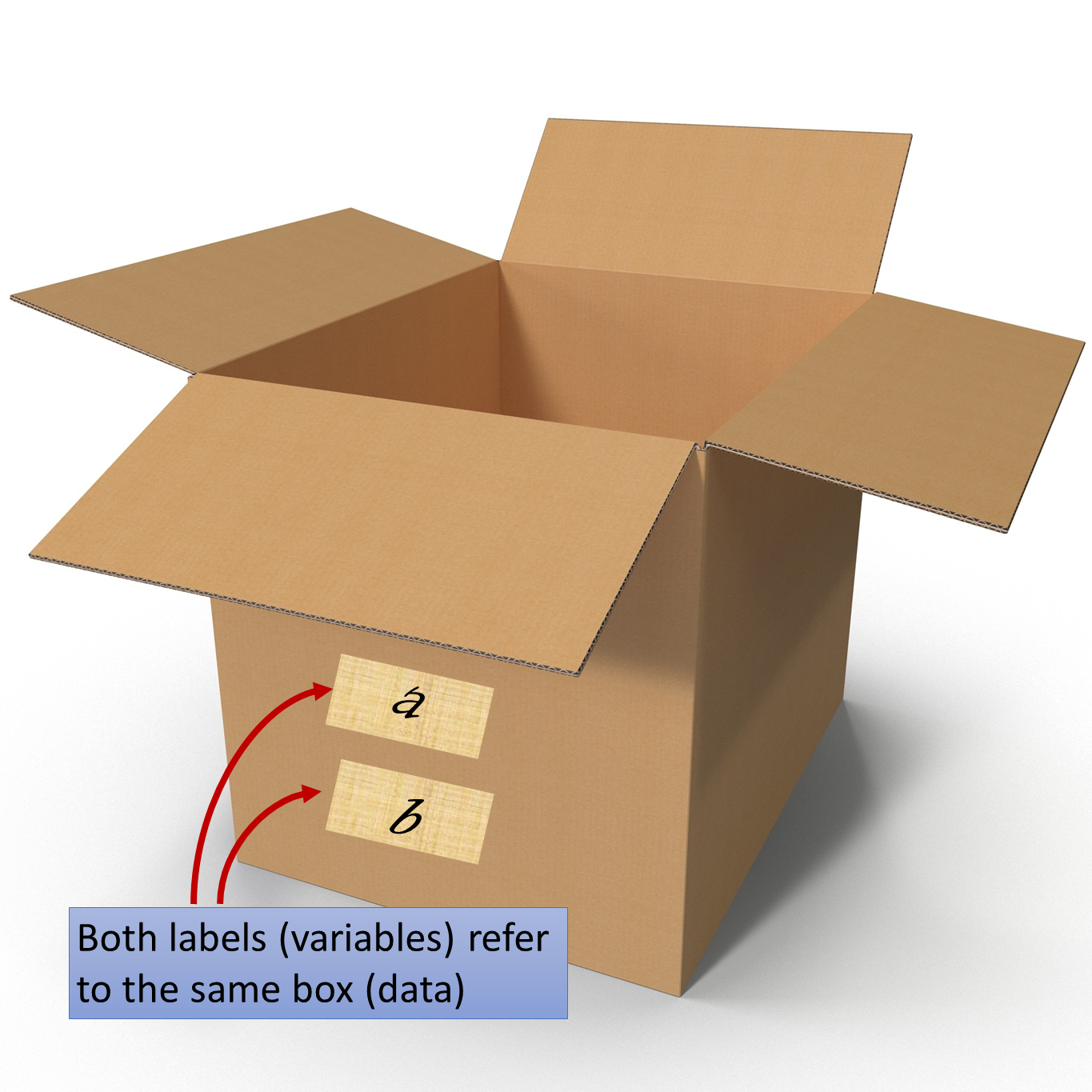
Variables Are Labels

One important thing to remember about variables is that they are labels for data, not the data itself. Let's illustrate what that means. At this point, a refers to a Vector. We will create another variable, b, and assign it the value of a.

julia> b = a
3-element Vector{Int64}:
 1
 2
 3

Now let's change one of the elements of b.

julia> b[1] = 100; b
3-element Vector{Int64}:
 100
   2
   3

We didn't change a, so it should be the same as before, right? Nope!

julia> a
3-element Vector{Int64}:
 100
   2
   3

What happened? Remember, a is just a label for some data (a Vector). When we created b, we created a new label for the same data. Both a and b refer to the same data, so modifying one modifies the other.

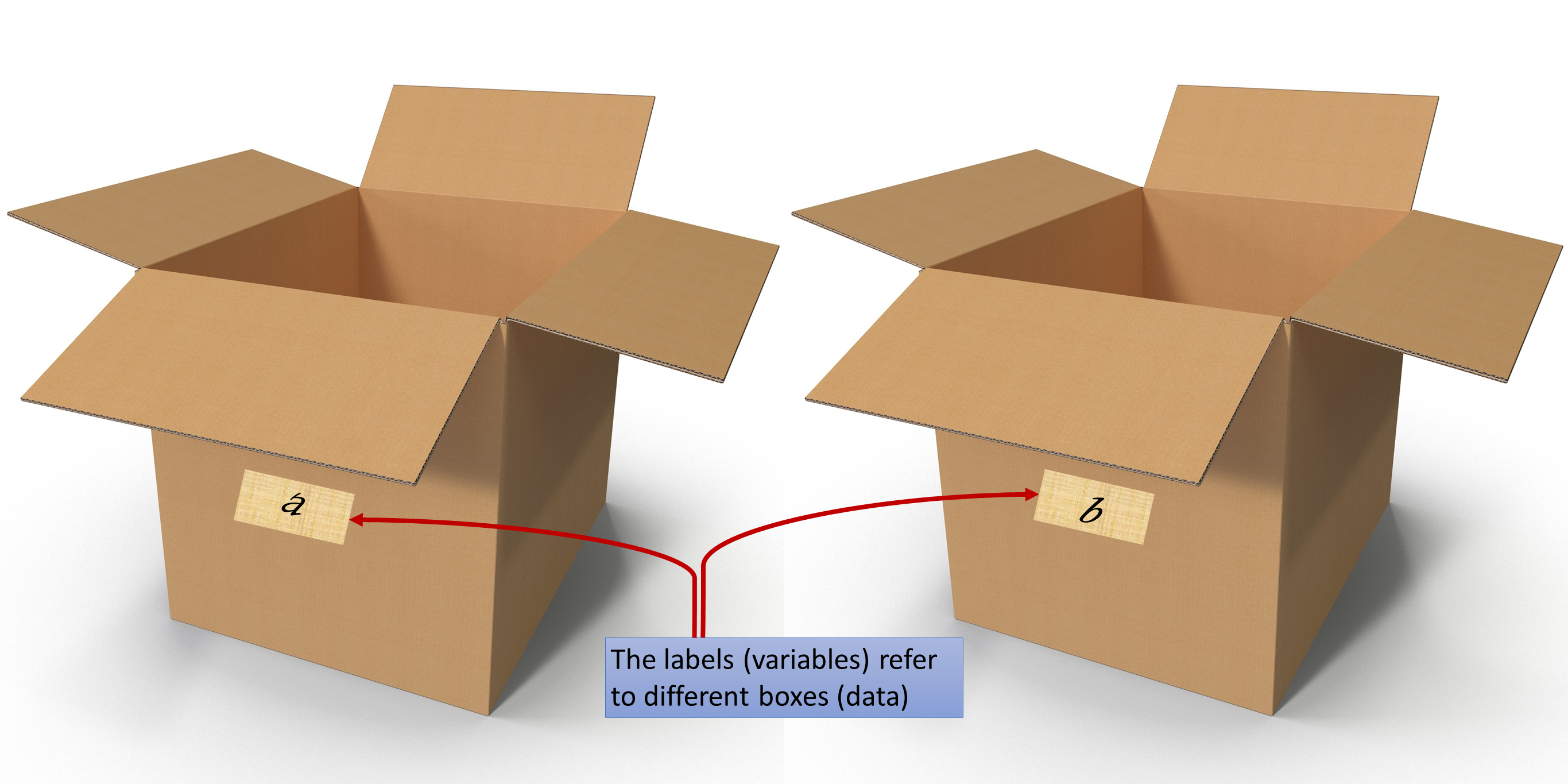
If you want b to have the same values as a but refer to different data, use copy.

julia> b = copy(a)
3-element Vector{Int64}:
 100
   2
   3

julia> b[1] = 1; b
3-element Vector{Int64}:
 1
 2
 3

julia> a
3-element Vector{Int64}:
 100
   2
   3

Now that we know how to create variables, let's learn about some basic types of data we can assign to variables.

Basic Types

Julia has many basic data types.

integer = 9000
floating_point = 3.14
boolean = true
imaginary = 1 + 2im
rational = 4//3
char = 'x'
str = "a string"
array = [1.0, 2.0]

Integers and floating-point numbers can be expressed with different numbers of bits.

Int64, Int32, Int16       # and more
Float64, Float32, Float16 # and more

By default, integer numbers (technically, literals) are of type Int64 on 64-bit computers or of type Int32 on 32-bit computers. (Note that Int is shorthand for Int64 or Int32 for 64-bit or 32-bit computers, respectively. Therefore, all integer literals are of type Int.)

On the other hand, floating-point numbers (literals) of the form 3.14 or 2.3e5 are of type Float64 on all computers, while those of the form 2.3f5 are of type Float32.

To use different numbers of bits, just use the appropriate constructor.

julia> Int16(20)
20

julia> Float16(1.2)
Float16(1.2)

Basic Operations

Now we will cover some basic operations. This is by no means an exhaustive list; check out the Julia documentation for more details.

# Math
addition = 1 + 2.0
subtraction = 1 - 1
multiplication = 3 * 4//3
division = 6 / 4
integer_division = 6 ÷ 4 # Type \div<tab>
power = 2^7

# Boolean
not = !false
and = true && not
or = not || and

# Comparison
equality = addition == 1
greater = division > integer_division
chained = addition < subtraction <= power

# Strings
string_concatenation = "hi " * "there"
string_interpolation = "1 - 1 = $subtraction"
string_indexing = string_interpolation[5]
substring = string_concatenation[4:end]
parsing = parse(Int, string_indexing)

# Arrays
a = [1, 2, 3]
b = [4, 5, 6]
concat_vert = [a; b]
concat_horiz = [a b]
vector_indexing = b[2]
vector_range_indexing = b[1:2]
matrix_indexing = concat_horiz[2:3,1]
elementwise1 = a .+ 1
elementwise2 = a .- b

# Displaying
print(addition)
println(string_concatenation)
@show not
@info "some variables" power a

Function Basics

Some of the basic operations we saw above, e.g., parse and print, were functions. As demonstrated above, functions are called using the following familiar syntax:

func()           # For no inputs
func(arg1)       # For one input
func(arg1, arg2) # For two inputs
# etc.

Note that just writing the function name (i.e., without parentheses) is valid syntax, but it is not a function call. In this case, the function name is treated essentially like a variable, meaning, for example, it can be used as an input to another function.

For example, one way to compute the sum of the absolute value of an array of numbers is as follows:

julia> sum(abs, [-1, 0, 1])
2

Here, the function abs is not being called (by us) but is used as an input to the function sum as if it were a variable.

Function Vectorization

Often, we have a function that operates on a single input that we want to apply to every element of an array. Julia provides a convenient syntax to do so: just add a dot (.). For example, the following takes the absolute value of every array element:

julia> abs.([-1, 0, 1])
3-element Vector{Int64}
 1
 0
 1

There is also a function, map, that does the same thing in this example:

julia> map(abs, [-1, 0, 1])
3-element Vector{Int64}
 1
 0
 1

(Note, however, that map and the dot syntax are not always interchangeable.)

Defining Functions

When writing Julia code, it is convenient to place code inside of functions. There are two main syntaxes for creating a function.

1. Using the function keyword:

   function myfunc(x)
       return x + 1
   end
   

2. Using the assignment form:

   myfunc2(x, y) = x + y
   

Optional Arguments

Sometimes we want a function to have optional inputs. The syntax for specifying optional arguments is

function myfunc3(required, optional = "hello")
    println(required, optional)
end

Here, optional is optional and has a default value of "hello" if not provided by the caller.

julia> myfunc3("say ")
say hello

julia> myfunc3("see you ", "later")
see you later

Keyword Arguments

Another way to specify optional arguments is to use keyword arguments. The syntax is almost the same as regular optional arguments, except we use a semicolon (;) instead of a comma (,).

function myfunc4(x; y = 3)
    return x * y
end

Here, y is optional, but to specify it we need to use the keyword y.

julia> myfunc4(2)
6

julia> myfunc4(2; y = 10)
20

julia> myfunc4(2, 10)
ERROR: MethodError: no method matching myfunc4(::Int64, ::Int64)

When calling myfunc4 we can also use a comma when specifying y.

julia> myfunc4(2, y = 1)
2

Returning Multiple Values

Sometimes we need a function to return multiple values. The way to do this in Julia is to return a Tuple. Here's an example:

function plusminus1(x)
    return (x + 1, x - 1)
end

Then multiple variables can be assigned at once.

julia> (plus1, minus1) = plusminus1(1)
(2, 0)

julia> plus1
2

julia> minus1
0

Note that taking the output of a function with multiple return values and assigning it to a single variable will assign that variable the whole Tuple of outputs. The following code illustrates this and shows how to return just one output:

julia> both = plusminus1(1);

julia> both
(2, 0)

julia> (one,) = plusminus1(1);

julia> one
2

(Note, however, that in this last case the second output is still computed; it is just immediately discarded, so there are no savings in computation.)

Vectorizing a Function with Multiple Return Values

Vectorizing a function with multiple return values requires a bit more work. For this example, we will use the sincos function that computes the sine and cosine simultaneously. We can still use the dot syntax, but we might be tempted to try the following:

julia> (s, c) = sincos.([0, π/2, π]);

julia> s
(0.0, 1.0)

julia> c
(1.0, 6.123233995736766e-17)

Here, s has the value of sincos(0), not the value of sin.([0, π/2, π]) like we might have expected.

Instead, we can do the following:

julia> sc = sincos.([0, π/2, π])
3-element Vector{Tuple{Float64, Float64}}:
 (0.0, 1.0)
 (1.0, 6.123233995736766e-17)
 (1.2246467991473532e-16, -1.0)

julia> s = first.(sc)
3-element Vector{Float64}:
 0.0
 1.0
 1.2246467991473532e-16

julia> c = last.(sc)
3-element Vector{Float64}:
  1.0
  6.123233995736766e-17
 -1.0

(Note that instead of using first or last, we could write it this way: output_i = getindex.(sc, i). This way also works for functions that return more than two values.)

Summary

In this post, we learned about what a variable is and some basic data types. We also learned about how to define and use functions.

There is a lot more we could cover about these topics, so if you want to learn more, check out the links below, or write a comment below letting us know what additional concepts or topics you would like to see!

Understand variables and functions in Julia? Move on to the next post to learn how to master the Julia REPL! Or, feel free to take a look at our other Julia tutorial posts!

Additional Links

• Julia documentation
  • For variables
  • For integer and floating-point numbers
  • For complex and rational numbers
  • For basic operations
  • For strings
  • For functions